Fourier coefficients of a 2D curve are generated with numerical integration and displayed as epicycles.

Epicycles

The associated Xcode project implements an iOS and macOS SwiftUI app that numerically calculates the Fourier series of sampled parametric curves (x(t), y(t)) in the plane, points drawn by the user, or the samples of finite Fourier series created with a terms editor.

Experiment with complex Fourier series of the form:

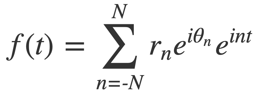
By Euler’s formula the n-th term (or frequency component) of the Fourier series is a complex number that traces a circle with radius r_n in the 2D plane n times as t traverses an interval (period) of length 2π. The values of the sum trace the path of the function f(t) as t traverses an interval (period) of length 2π:

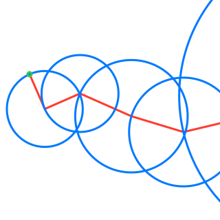
The circles in these animations that rotate on top of other circles are called epicycles. Each epicycle corresponds to a term of the complex Fourier series. The origin is at the constant term n = 0.

The partial sums of the Fourier series are used to draw the red line segment path in the animations, and also locate the centers of each blue epicycle circle. The radius of each epicycle circle is the magnitude of its corresponding Fourier series coefficient:

The origin of every red line segment path is determined by the constant term of the Fourier series, n = 0, and is fixed in time.

The end of every red line segment path is the value of the whole Fourier series, and is located at the green circle in the animations:

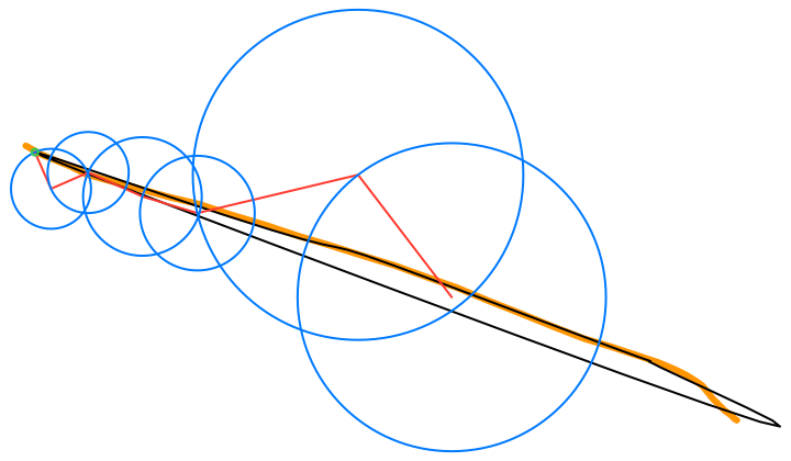
The green circle follows the approximating curve of the Fourier series, drawn in black over the orange curve of the function f(t):

Epicycles Index

Euler’s Formula and the Unit Circle
Complex Fourier Series
Complex Fourier Series Example
Derive Fourier Series Coefficients
Numerical Calculation of Fourier Series Coefficients

Euler’s Formula and the Unit Circle

Epicycles Index ↑

The measure θ of an angle is defined to be the arc length a it subtends on the unit circle, θ = a:

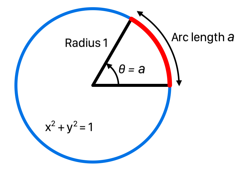
The unit of measure for angles is the radian, which is the angle that subtends an arc length of 1 on the unit circle, denoted by rad.

For a circle with radius r the total arc length C of its circumference is given by C = 2πr. Thus C = 2π for the unit circle, and a radian is the fraction 1/(2π) of its circumference C. A radian subtends the same fraction 1/(2π) of the circumference C of any other circle. But r = C/(2π), so a radian subtends an arc length r on a circle with radius r, hence the name radian.

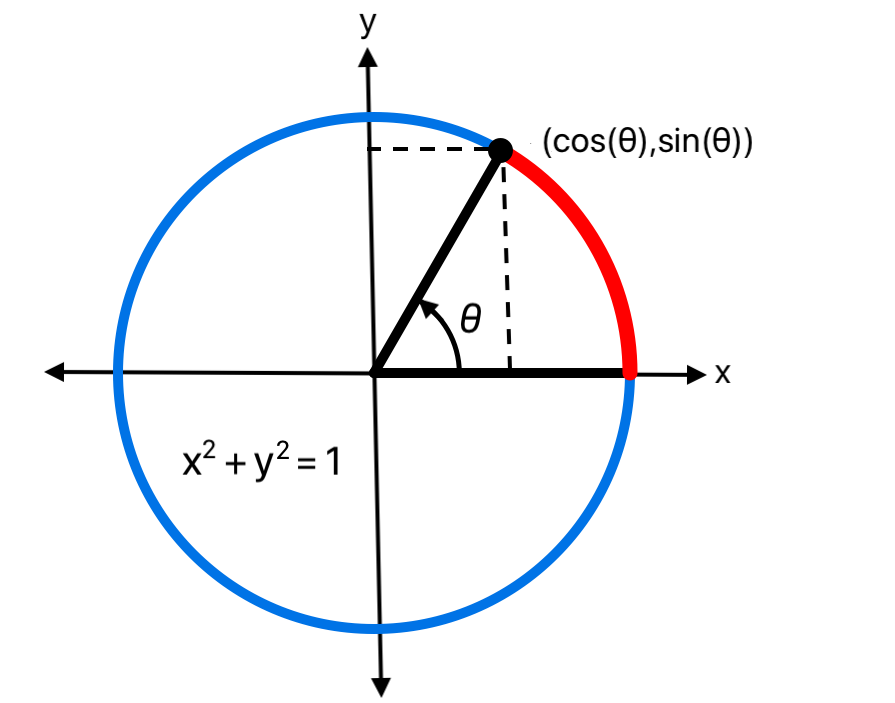
The trigonometric sine and cosine functions are defined as the coordinates on the unit circle determined by the angle θ:

Euler’s Formula connects the trigonometric functions to the complex exponential:

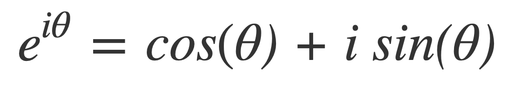
Where i is the imaginary unit : i² = −1

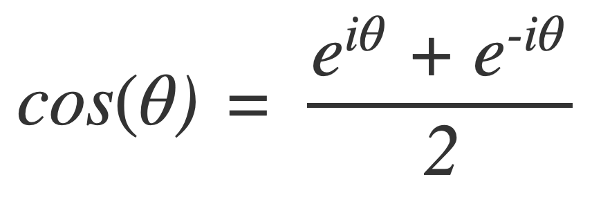
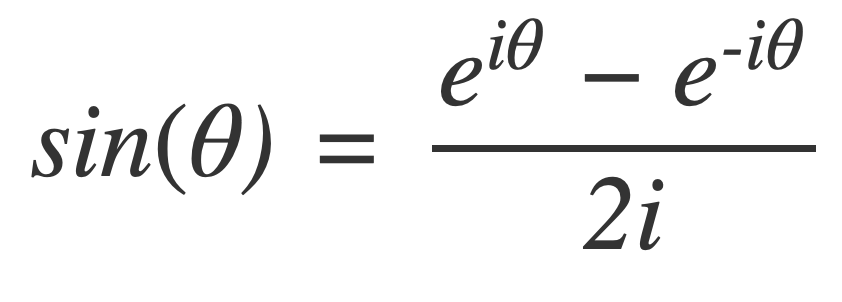
The trigonometric functions can be expressed in terms of the complex exponential function:

A complex number c = x + i y, that corresponds to a coordinate point (x,y) in the 2D plane, can be expressed in the polar form of a complex number r e^iθ. The angle θ is called the argument of the complex number c. The factor r is the modulus (magnitude, or amplitude) of the complex number.

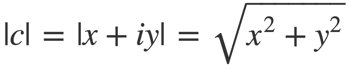
The modulus |c| of a complex number c = x + i y is a real number that is its distance from the origin, given by:

Since the complex exponential satisfies the following exponential law, complex multiplication is a rotation with scaling. When multiplying complex numbers in this form the exponents add (rotation) and the magnitudes multiply (scaling):

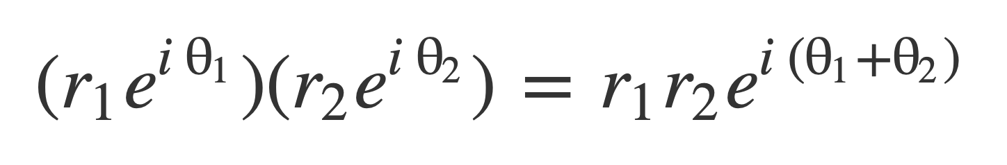
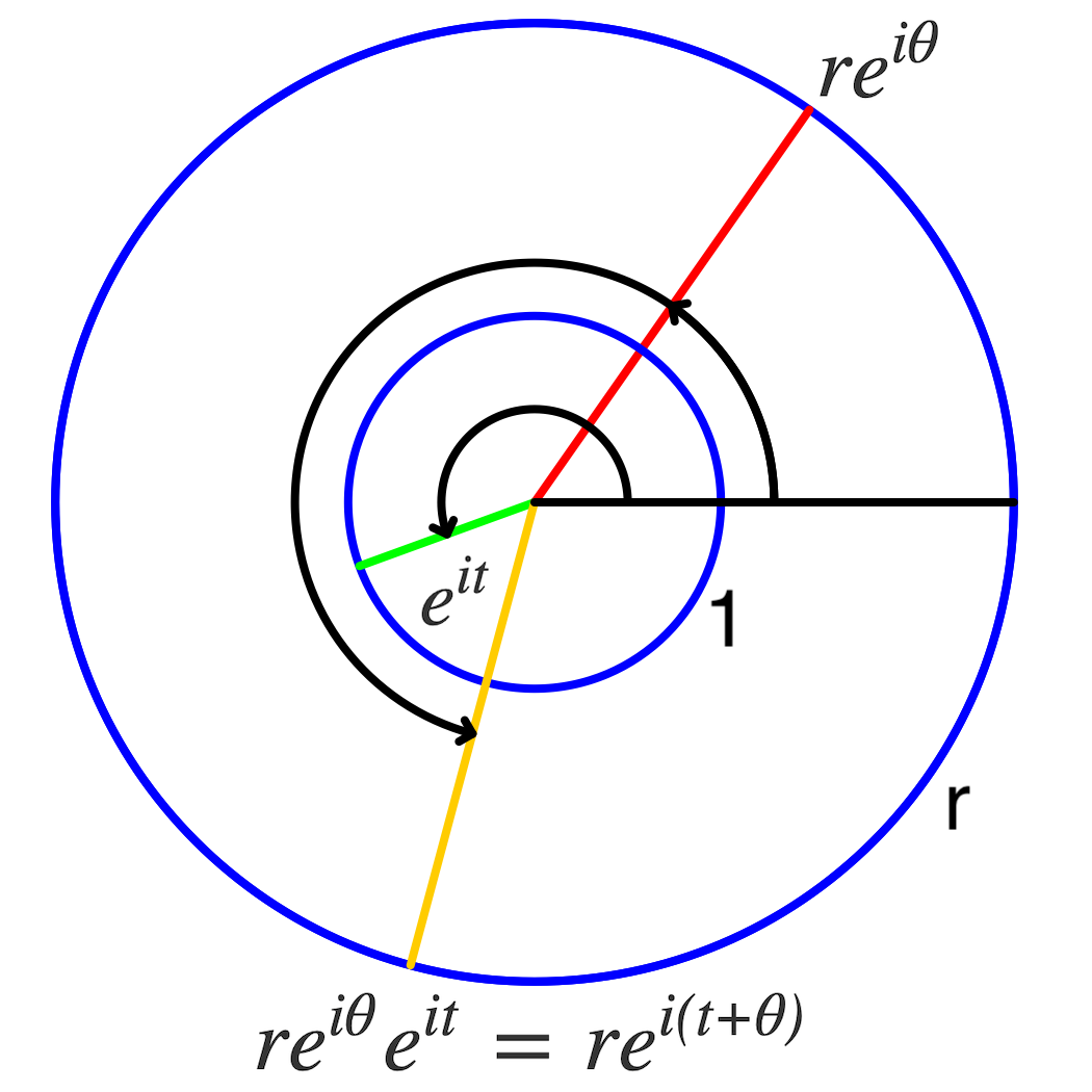
The point e^it has magnitude of 1, and as t traverses the interval [-π, π] from -π to π, the point e^it rotates around the unit circle one time, while the point r e^iθ e^it rotates around a circle of radius r one time.

For any integer n, the point r e^{i n t} rotates around a circle of radius r, n times as t traverses the interval [-π, π] from -π to π. The sign of n determines direction of rotation: -n rotates in the opposite direction of n.

Complex Fourier Series

Epicycles Index ↑

A non-constant function f with the property f(t + c) = f(t) for a some constant c and all t is said to be periodic, and the period is the smallest such c.

The sine and cosine functions are periodic, with period 2π, by their definition using the unit circle, with an angle defined as arc length.

Frequency is then defined in either oscillatory or angular units:

• Oscillatory frequency f is cycles per second, labelled hertz or Hz. For a periodic function with period k, oscillatory frequency f is f = 1/k, the number of periods in the unit interval [0,1].

• Angular frequency ω is the corresponding radians per second given by ω = 2πf, so 1 Hz (1 cycle per second) corresponds to 1 full angular revolution, or 2π radians per second.

If a periodic complex valued function f(t) = (x(t), y(t)) = x(t) + i y(t) with period 2π satisfies conditions for pointwise convergence then it may be represented by the following expression, a Fourier Series:

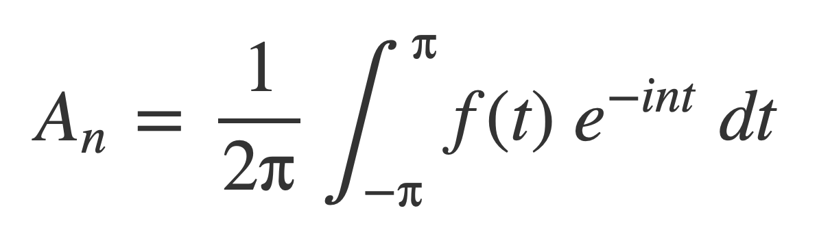
With the complex coefficients given by:

The Fourier series is a sum of frequency components e^{i n t} with complex valued weights given by A_n (any of which may be zero).

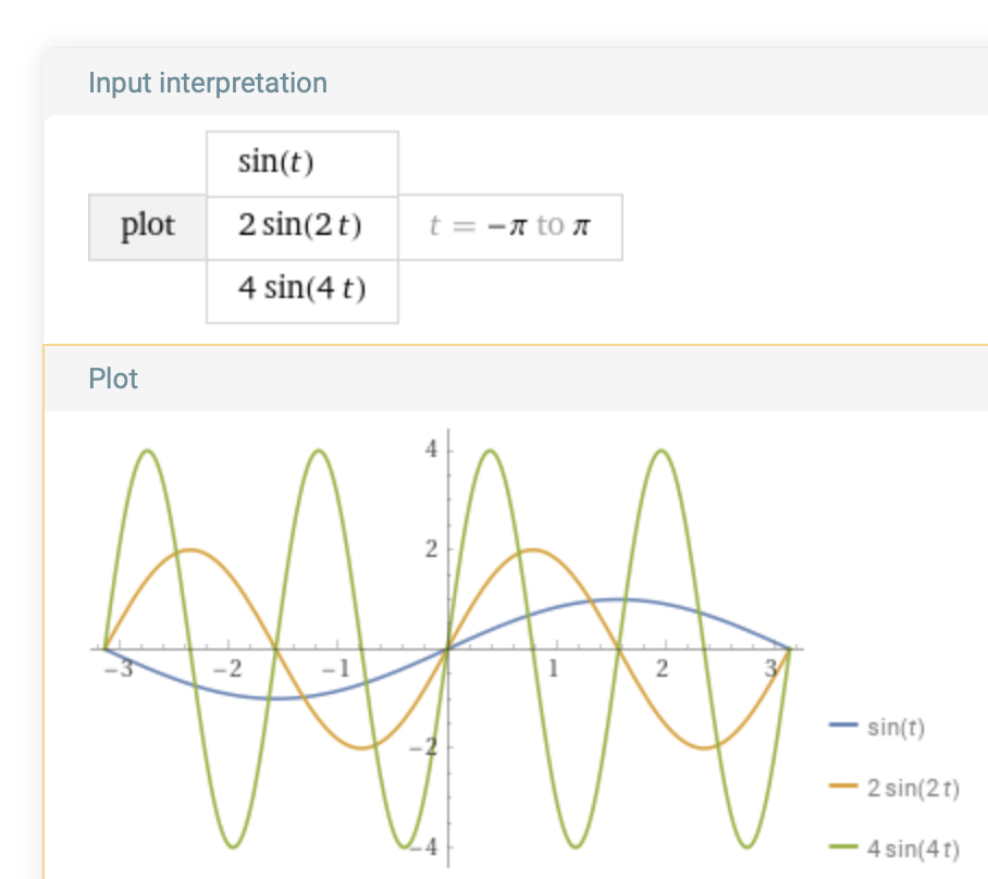
Since sine and cosine can be represented in terms of the complex exponential, this leads to the result that a periodic function f(t) with period 2π may be decomposable into a weighted sum of sin(nt) and cos(nt), with angular frequencies that are positive integers n= 1,2,3,…

Here is a plot of some sin(nt) functions whose angular frequencies n=1,2,4 are multiples of one another:

plot sin t with 2 sin 2t with 4 sin 4t on -π,π

The coefficients A_n will be evaluated by sampling the integrands f(t) e^{-i n t} on a uniformly spaced grid and using the Simpson’s Rule method of numerical integration.

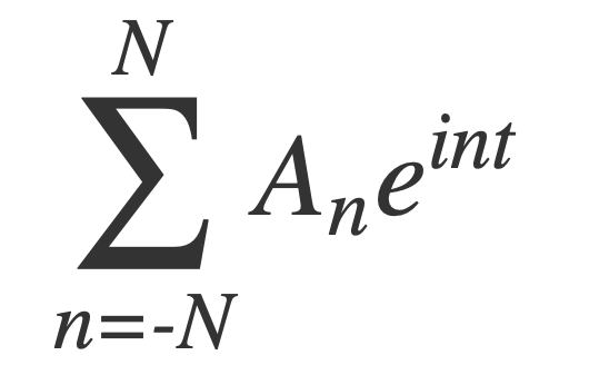
Note that the summation is for n = -∞ to ∞, hence contains positive and negative values of n. So in practice partial sums of finite subsequences of the 2N+1 terms is actually summed in alternating order, beginning with 0: 0,1,-1,2,-2,3,-3,…

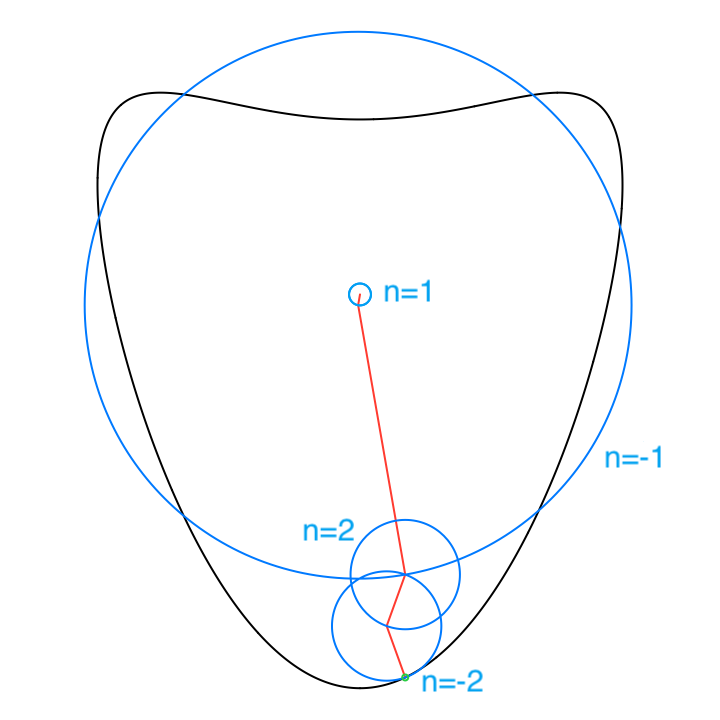
This way a 2D curve, represented by a complex valued function f(t) = (x(t), y(t)) = x(t) + i y(t), can be visualized as a chain of epicycles, or circles upon circles, with each of the circles corresponding to a component A_ne^{i n t} of the complex Fourier series, beginning at the origin given by A₀:

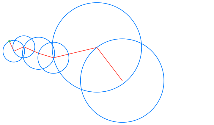
The modulus of a coefficient A_n, a complex number, is the radius of the nth circle that is traced as the multiplication by e^{i n t} rotates A_n, n time as time t traverses the period [-π, π]. The rotational direction of terms n and -n oppose one another. The term n = 0 is a single constant point, that does not rotate at all, and serves as the origin of the summation illustration.

If N is the desired number of terms chosen for the Fourier series, the red segmented line at time t in the above diagram is generated as follows by computing partial sums for n = 0,1,-1,2,-2,…,N,-N, implemented by the function fourierSeriesEpicyclePoints, described in Calculate Fourier Series:

n = 0 : The constant term A₀, is the origin where drawing begins.
n = 1 : The first line segment is then drawn from the origin A₀ to A₀ + A₁ e^{i t}.
n = -1 : The second line segment is then drawn from the end of the first line segment at A₀ + A₁ e^{i t} to A₀ + A₁ e^{i t} + A_-1 e^{-i t}.
Continue this way to n = -N, ending with the total sum value of the Fourier series at time t, located at the green circle in the above diagram, the approximating value for f(t).

Of course some of the coefficients A_n may be zero.

The following animated illustrations of Fourier series were created with the Terms editor. Each Fourier series has two frequency component terms. In the top table row the Fourier series frequency components are {1,2}, {1,3} and {1,4}, and the outer radius rotates 2,3 and 4 times for each rotation of the inner radius. In the bottom table row the components are the negated versions of the top row, namely {-1,-2}, {-1,-3} and {-1,-4}, and the outer radius still rotates 2,3 and 4 times for each rotation of the inner, but rotation of each term is in the opposite direction of the corresponding term in the top table row.

n=1,2

n=1,3

n=1,4

n=-1,-2

n=-1,-3

n=-1,-4

Here is an example with n = 1,-1,2,-2 - don’t miss the the very small circle at the center! Look closely at the direction the radii of the circles are rotating in the animations to see how they alternate direction. This is because the series is ordered as follows, with n = 0 the origin point (or degenerate circle):

n = 0, 1, -1, 2, -2, …

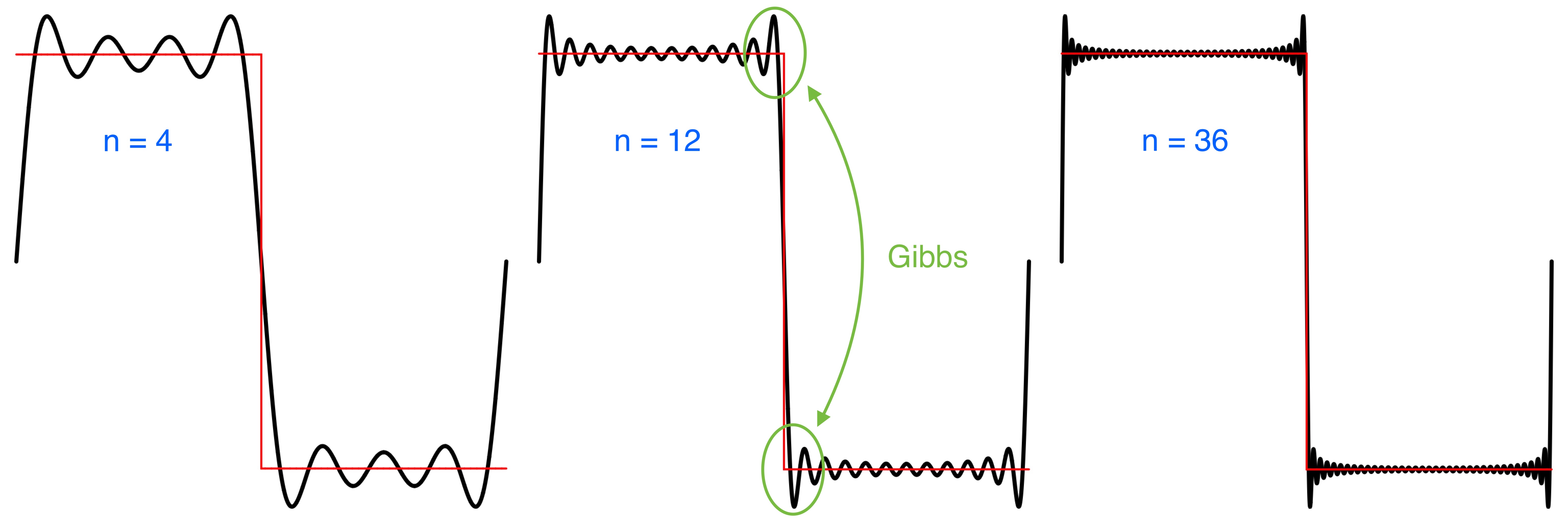
Pointwise convergence of Fourier series occurs at points where the function is differentiable, except for the Gibbs phenomenon at discontinuities.

Plotting the Fourier series for varying number of terms illustrates how the approximation improves with more terms, except near the discontinuities where the overshoot remains. The square wave plotted in red, the Fourier series in black, various number of terms n.

Complex Fourier Series Example

Epicycles Index ↑

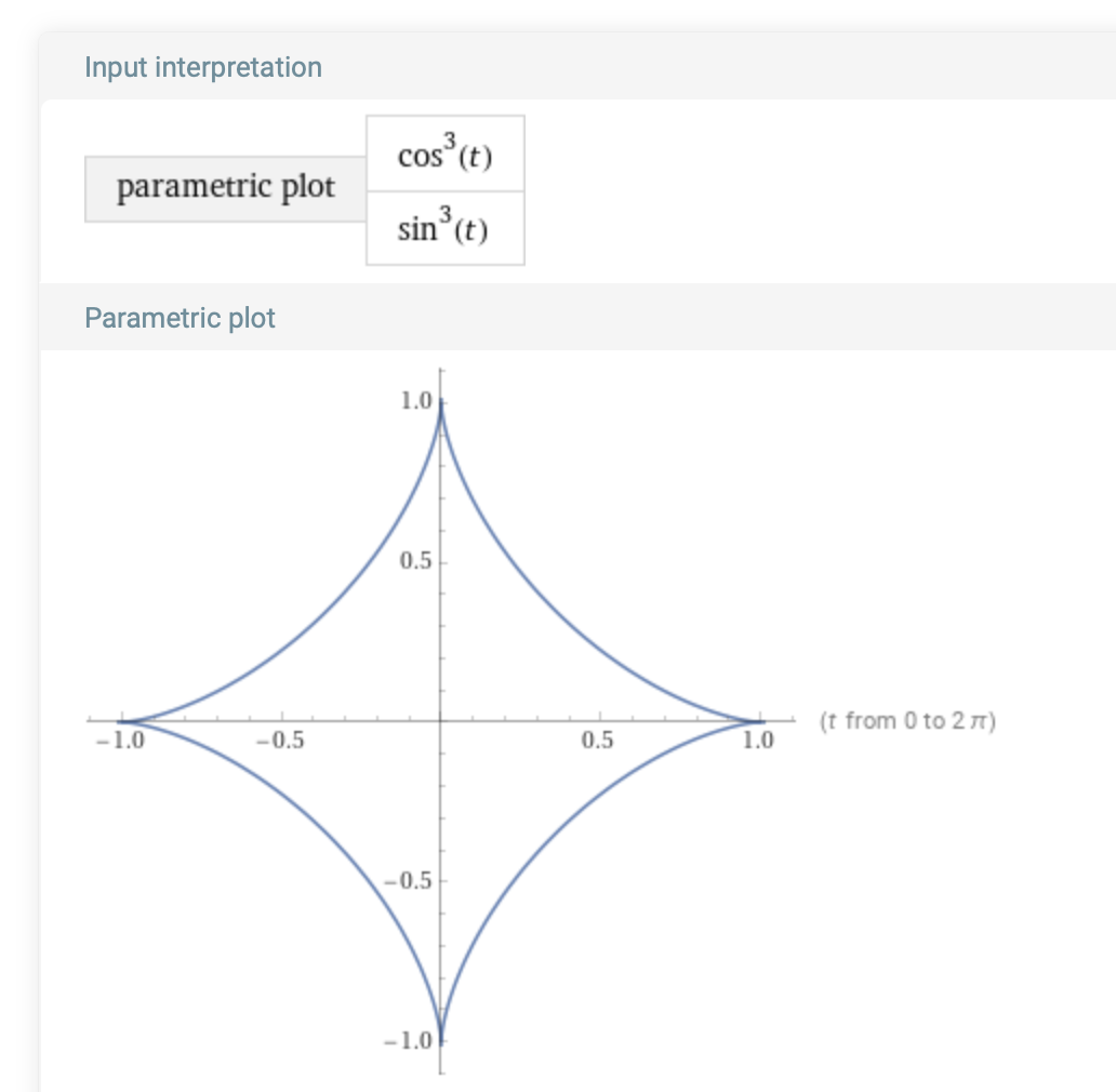
The Astroid curve, a pinched in circle, in 2D parametric form is given as, t in [-π,π] :

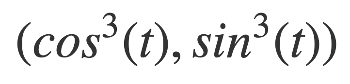
Plot it with:

parametric plot (cos^3 t, sin^3 t)

The Fourier series can be calculated with:

FourierSeries[(Power[cos(t),3],Power[sin(t),3]),t,3]

Combine the result into the form of a complex series:

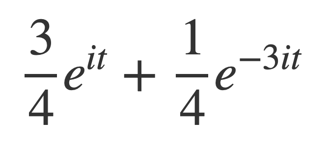
Using Euler’s formula this is equivalent to the parametric equations:

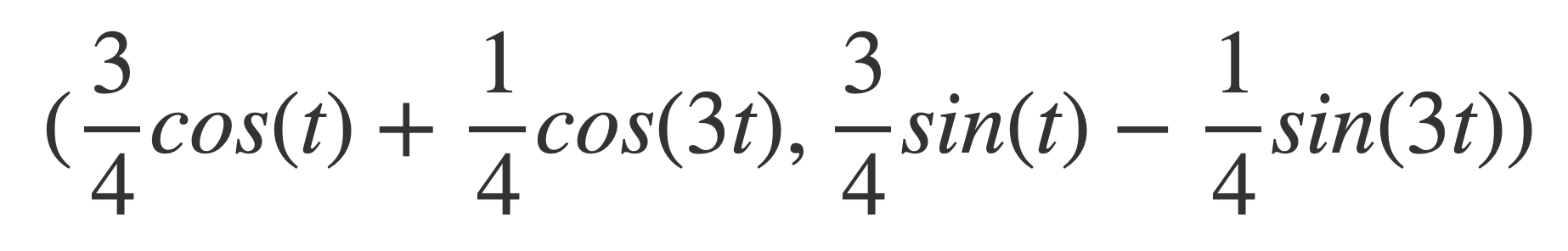
Using Multiple-Angle Formulas for sin(t) and cos(t), and the Pythagorean trigonometric identity, these can be expressed as the original parametric equations:

In the Epicycles app tap the ? function type, select the Terms tab, and enter the corresponding terms of the astroid’s Fourier series.

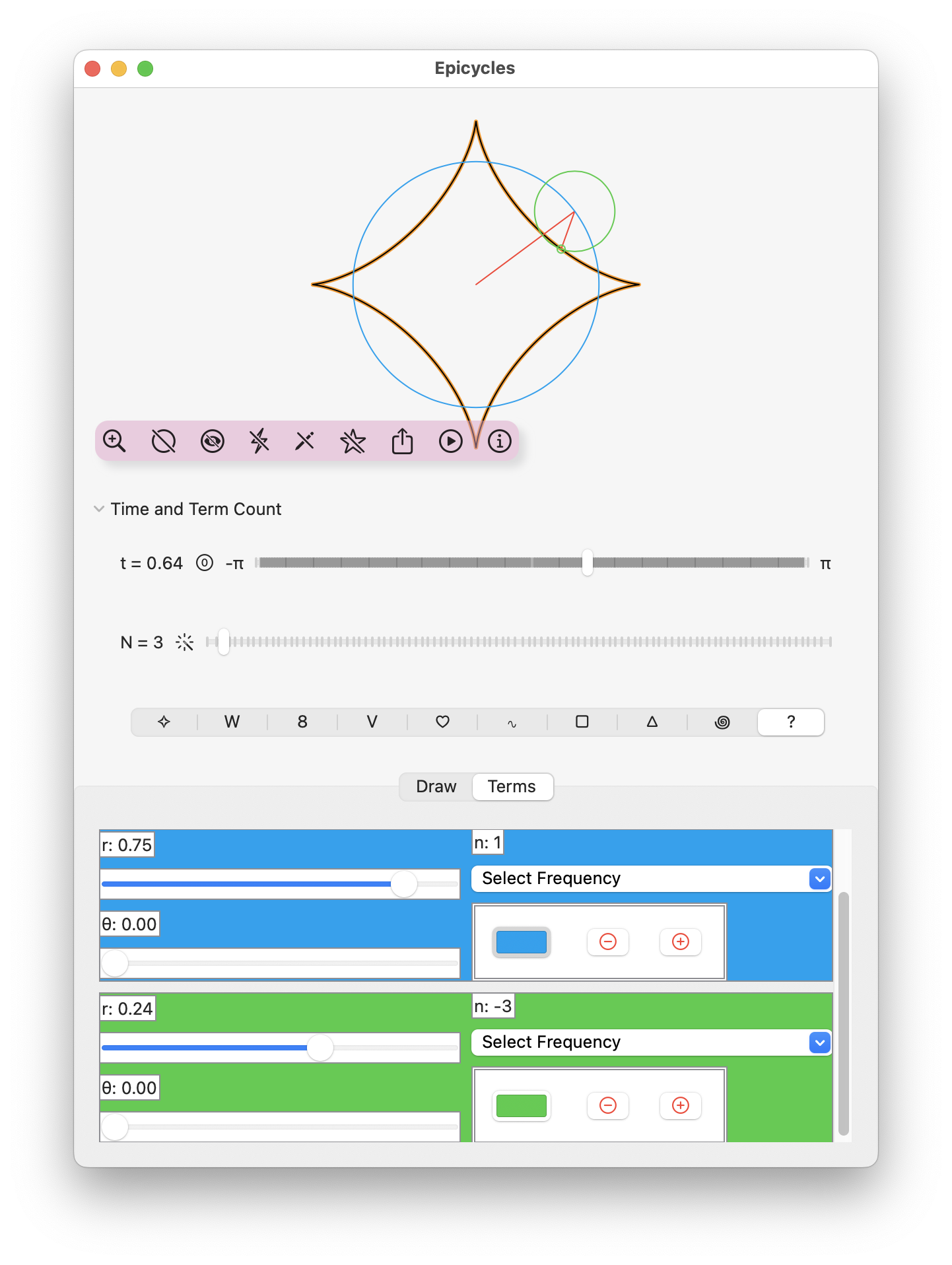
Namely terms {r = 0.75, θ = 0, n = 1} and {r = 0.25, θ = 0, n = -3}.

Tap the share button In the Graphic Menu:

And export a GIF animation:

Derive Fourier Series Coefficients

Epicycles Index ↑

The formula for the coefficients of the Fourier series can be derived using a few properties of the sin and cos functions.

On the interval [-π,π] functions sin(t) and cos(t) look like this:

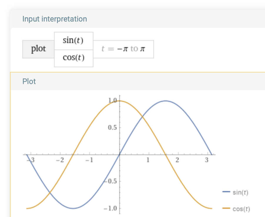
For all non-zero integers n:

cos(-nπ) = cos(nπ)

sin(-nπ) = sin(nπ) = 0

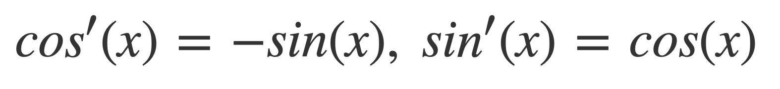
The derivatives of cos and sin are given by:

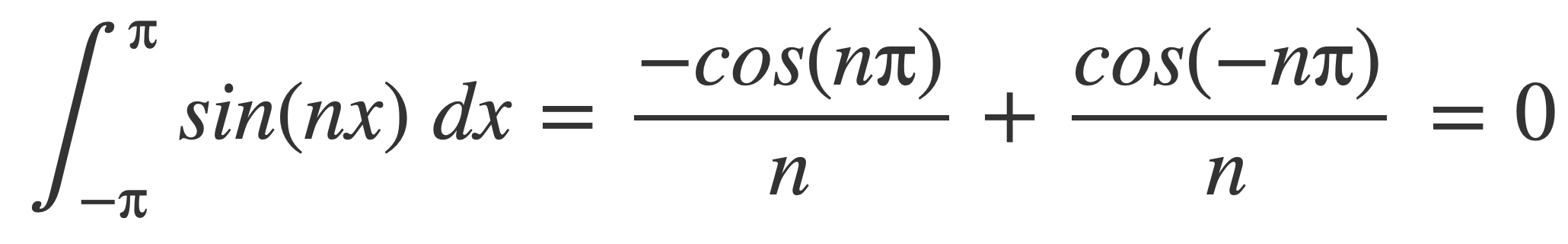
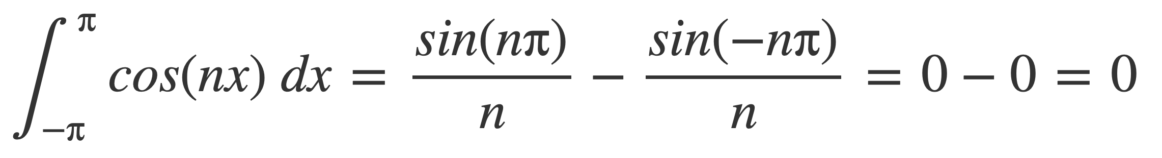
Use this to apply the fundamental theorem of calculus to find that these integrals evaluate to zero for all non-zero integers n:

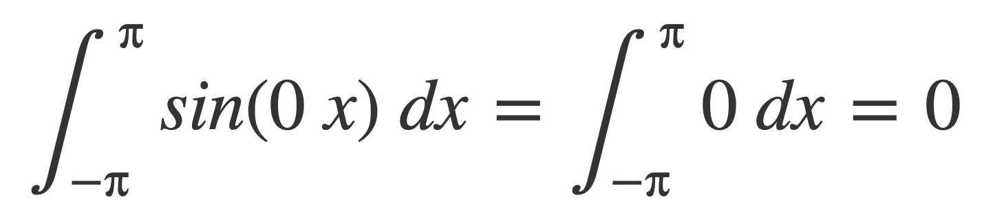
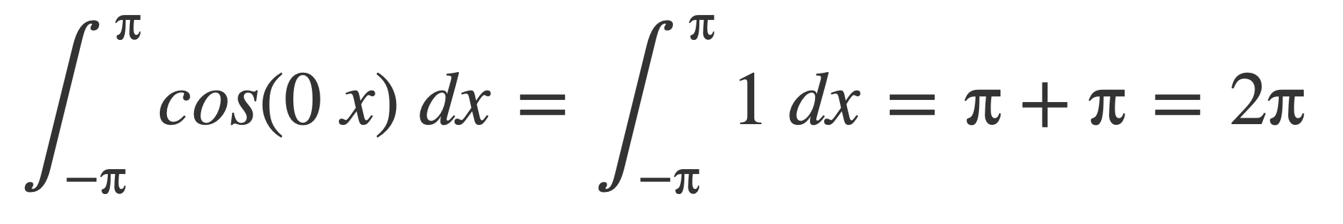
Also, if n = 0:

Let the symbol δ_mn represent 0 when m ≠ n, and 1 when m = n. Then for any integers m and n:

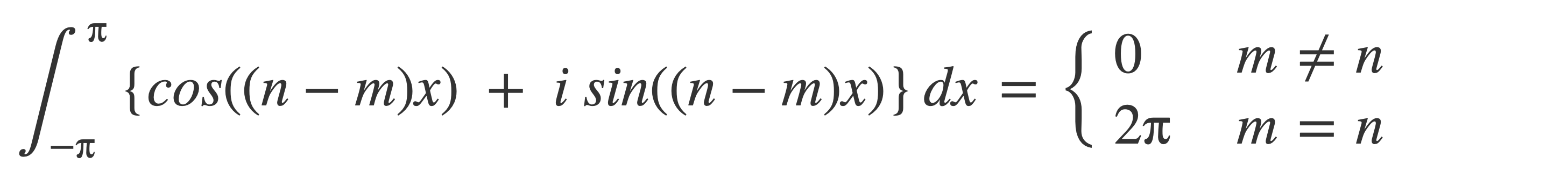
So, by Euler’s formula, for any integers m and n:

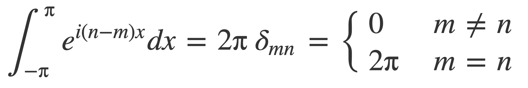
This final result is useful for the following calculation to derive the coefficients of the Fourier series.

Suppose that f(t) is defined by the following expression, namely the Fourier series:

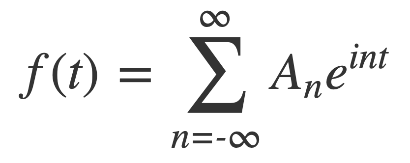
To derive the expression for the coefficient A_n, multiply each side of this expression by e^-imt, and integrate each side over [-π,π], applying previous results:

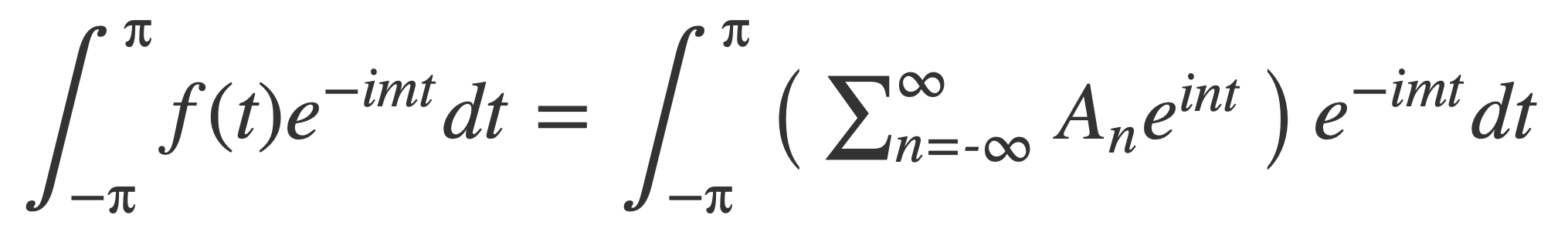
Therefore the complex coefficients A_n are given by:

Numerical Calculation of Fourier Series Coefficients

Epicycles Index ↑

A complex number p is represented by a 2-tuple p:(Double, Double), for the complex number p.0 + i p.1.

Math Index

Complex Addition
Complex Multiplication
Complex Exponential
Numerical Integration
Function Samples

Hardcoded Functions

Custom Fourier Series
Calculate Fourier Coefficients
Calculate Fourier Series

Complex Addition

Math Index

The addition rule for complex numbers (x + i y) + (u + i v) = (x + u) + i (y + v) is implemented by complexAdd:

func complexAdd(_ a:(Double,Double), _ b:(Double,Double)) -> (Double,Double) {
        //  (x   + y   i)(u   + v   i) = (x   + u  ) + (y   + v  )i
        //  (a.0 + a.1 i)(b.0 + b.1 i) = (a.0 + b.0) + (a.1 + b.1)i
    
    return (a.0 + b.0, a.1 + b.1)
}

Complex Multiplication

Math Index

The multiplication rule for complex numbers (x + y i) • (u + v i) = (xu - yv) + (xv + yu) i is implemented by complexMultiply:

func complexMultiply(_ a:(Double,Double), _ b:(Double,Double)) -> (Double,Double) {
        //  (x   + y   i)(u   + v   i) = (x   u   - y   v  ) + (x   v   + y   u  )i
        //  (a.0 + a.1 i)(b.0 + b.1 i) = (a.0 b.0 - a.1 b.1) + (a.0 b.1 + a.1 b.0)i
    
    return (a.0 * b.0 - a.1 * b.1 , a.0 * b.1 + a.1 * b.0)
}

Complex Exponential

Math Index

The nth complex exponential e^int is implemented by e, and the related sin and cos:

func e(_ t:Double, _ n:Double) -> (Double,Double) {
    return (cos(n * t), sin(n * t))
}

func cos(_ n:Int, sampleCount:Int) -> [Double] {
    return sample(sampleCount: sampleCount) { t in
        cos(Double(n) * t)
    }
}

func sin(_ n:Int, sampleCount:Int) -> [Double] {
    return sample(sampleCount: sampleCount) { t in
        sin(Double(n) * t)
    }
}

Numerical Integration

Math Index

The integrals that define the Fourier coefficients A_n of a function are evaluated by the Simpson’s Rule algorithm, using the Accelerate framework method vDSP_vsimpsD, using the function’s samples.

func integrate(samples:[Double]) -> Double {
    
    let sampleCount = samples.count
    var step = (2 * .pi) / Double(sampleCount-1)
    
    var result = [Double](repeating: 0.0, count: sampleCount)
    
    vDSP_vsimpsD(samples, 1, &step, &result, 1, vDSP_Length(sampleCount))
    
    return result[sampleCount-1]
}

Function Samples

Math Index

Samples for numerical integration are provided either by sampling a function f(t), parameterized by time t in the interval [-π, π], or directly from the points drawn in a view.

Functions f(t) are either:

Hardcoded functions, identified by the type Curve, which the user selects from a control, and provided as a tuple (x(t), y(t)) with a lookup function curveLookup, sampled with a function sample.
Custom Fourier series constructed from an array of structs of type Term the user creates in the terms editor, sampled with a function sampleTerms.

Hardcoded Functions

Math Index

Hardcoded functions f(t) = (x(t), y(t)) are identified by a Curve type. A lookup function curveLookup for a Curve returns a 2-tuple of functions (((Double)->Double), ((Double)->Double)) specifying (x(t), y(t)) for t the interval [-π, π].

struct Curve: Hashable, Identifiable {
    let id = UUID()
    let name: String
}

let curves: [Curve] = [
    Curve(name: "✧"),
    Curve(name: "W"),
    Curve(name: "8"),
    Curve(name: "V"),
    Curve(name: "♡"),
    Curve(name: "∿"),
    Curve(name: "□"),
    Curve(name: "△"),
    Curve(name: "꩜"),
    Curve(name: "?"),
]

func curveLookup(curve:Curve) -> (((Double)->Double), ((Double)->Double)) {
    var x:((Double)->Double)
    var y:((Double)->Double)
    
    let curveIndex = curves.firstIndex(of: curve)!+1
    
    switch curveIndex {
        case 1: // Astroid 7
            x = { t in pow(cos(t),7) }
            y = { t in pow(sin(t),7) }
        case 2: // Wave
            x = { t in pow(3 * t,2) }
            y = { t in 15 * t * cos(4 * t) }
        case 3: // Loop
            x = { t in t * t * sin(t) * cos(t) }
            y = { t in t * cos(t/2) }
        case 4: // V
            x = { t in pow(t,3)}
            y = { t in pow(2 * t,2)}
        case 5: // Heart
            x = { t in 16 * pow(sin(t),3) }
            y = { t in 13 * cos(t) - 5 * cos(2 * t) - 2 * cos(3 * t) - cos(4 * t) }
        case 6: // sine
            x = { t in t }
            y = { t in wavefunction(t + .pi, 1.0 / (.pi), .pi / 2, 0, .sine) }
        case 7: // square
            x = { t in t }
            y = { t in wavefunction(t + .pi, 1.0 / (.pi), .pi / 2, 0, .square) }
        case 8: // triangle
            x = { t in t }
            y = { t in wavefunction(t + .pi, 1.0 / (.pi), .pi / 2, 0, .triangle) }
        case 9: // Archimedean spiral
            x = { t in (t + .pi) * cos(3 * (t + .pi)) }
            y = { t in (t + .pi) * sin(3 * (t + .pi)) }
        default: // circle
            x = { t in cos(t) }
            y = { t in sin(t) }
    }
    
    return (x,y)
}

These curves are uniformly sampled on the interval [-π, π], with the function sample:

func sample(sampleCount:Int, f: (Double)->Double) -> [Double] {
    let step = (2 * .pi) / Double(sampleCount-1)
    let samples = stride(from: 0, through: sampleCount-1, by: 1).map { f(Double($0) * step - .pi) } // samples.count = sampleCount
    return samples
}

Custom Fourier Series

Math Index

A custom Fourier series is an array [Term] with elements of the form:

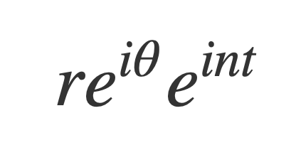
Each element r e^iθ e^int is a complex valued function of t on the interval [-π, π], represented by a Term struct, that specifies the amplitude r and phase θ for the coefficient of the term in polar form of a complex number, and its frequency component n.

struct Term: Identifiable, Equatable, Codable {
    let id = UUID()
    var amplitude: Double // -1...1
    var phase: Double // 0...2 * .pi
    var frequencyComponent: Int // -20...20

  ...

Given an array [Term], the function f(t) = (x(t), y(t)) it represents is the just sum of the terms, and it is uniformly sampled with the function sampleTerms, using complexAdd and complexMultiply :

func sampleTerms(sampleCount:Int, terms:[Term]) -> [CGPoint] {
    
    if terms.count == 0 {
        return []
    }
    
    var points:[CGPoint] = [CGPoint](repeating: .zero, count: sampleCount)
    
    let step = (2 * .pi) / Double(sampleCount-1)
    
    for i in 0...sampleCount-1 {
        let t = Double(i) * step - .pi
        var sum:(Double,Double) = (0,0)
        for term in terms {
            var An:(Double,Double)
            An = (term.amplitude * cos(term.phase), term.amplitude * sin(term.phase)) 
            let eint = e(t, Double(term.frequencyComponent))
            sum = complexAdd(sum, complexMultiply(An, eint))  
        }
        
        points[i] = CGPoint(x: sum.0, y: sum.1) 
    }
    
    return points
}

Calculate Fourier Coefficients

Math Index

The following integral for Fourier coefficients A_n is numerically computed using the samples for f(t) = (x(t),y(t)) and e(t,n):

Given two arrays x and y of [Double] for the sample values of the function f(t), its nth Fourier coefficient is calculated with fourierCoeffient_xy, that returns a 2-tuple for its complex value.

The calculation requires four numerical integrations. Using the trigonometric expression of the complex exponential (Euler’s Formula), the integrand is:

(x(t) + i y(t)) * (cos(n t) - i sin(n t))

The complex multiplication yields four integrands to be computed:

x(t) * cos(n t)

x(t) * sin(n t)

y(t) * cos(n t)

y(t) * sin(n t)

First, the cos(nt) and sin(nt) functions need to be sampled:

let cosn = cos(n, sampleCount: sampleCount)
let sinn = sin(n, sampleCount: sampleCount)

The multiplications for four integrands using the samples arrays (vectors) x,y,cosn and sinn are computed using the Accelerate framework method vDSP.multiply, which computes an elementwise product of a vector and a vector:

vDSP.multiply(x, cosn)

vDSP.multiply(x, sinn)

vDSP.multiply(y, cosn)

vDSP.multiply(y, sinn)

The arrays output from vDSP.multiply are passed to integrate, which performs the numerical integration:

cx.0 = (1.0/(.pi * 2)) * integrate(samples: vDSP.multiply(x, cosn))
cx.1 = -(1.0/(.pi * 2)) * integrate(samples: vDSP.multiply(x, sinn))
cy.0 = (1.0/(.pi * 2)) * integrate(samples: vDSP.multiply(y, cosn))
cy.1 = -(1.0/(.pi * 2)) * integrate(samples: vDSP.multiply(y, sinn))

The result is combined into a complex number as a 2-tuple, returned as the value of the coefficient A_n:

(cx.0 + i cx.1) + i (cy.0 + i cy.1) = cx.0 + i cx.1 + i cy.0 - cy.1 = (cx.0 - cy.1) + i (cx.1 + cy.0)

Or:

(cx.0 - cy.1, cx.1 + cy.0)

The complete function for computing A_n:

func fourierCoeffient_xy(n:Int, x:[Double], y:[Double]) -> (Double, Double) {
    var cx:(Double, Double) = (0,0)
    var cy:(Double, Double) = (0,0)
    
        // An = (1/2π) ∫ f(t)e^(-int) dt, [-π,π] 
        // e^(-int) = cos(n t) - i sint(n t)
        //
        // cx(n) = (1/(2π) ∫ x(t) e^(-i n t), [-π,π] 
        // cy(n) = (1/(2π) ∫ y(t) e^(-i n t), [-π,π] 
    
    let sampleCount = x.count
    
    let cosn = cos(n, sampleCount: sampleCount)
    let sinn = sin(n, sampleCount: sampleCount)
    
        // cx(n) = cx.0 + i cx.1
    cx.0 = (1.0/(.pi * 2)) * integrate(samples: vDSP.multiply(x, cosn))
    
    cx.1 = -(1.0/(.pi * 2)) * integrate(samples: vDSP.multiply(x, sinn))
    
        // cy(n) = cy.0 + i cy.1
    cy.0 = (1.0/(.pi * 2)) * integrate(samples: vDSP.multiply(y, cosn))
    
    cy.1 = -(1.0/(.pi * 2)) * integrate(samples: vDSP.multiply(y, sinn))
    
        // return as a complex number tuple
    /*
     (cx.0 + i cx.1) + i (cy.0 + i cy.1)
     = cx.0 + i cx.1 + i cy.0 - cy.1
     = (cx.0 - cy.1) + i (cx.1 + cy.0)
     */
    return (cx.0 - cy.1, cx.1 + cy.0)
}

Calculate Fourier Series

Math Index

To compute the Fourier series itself, all the Fourier coefficients A_n are computed for the selected number of terms N with the function fourierCoeffients_xy, note the plural form to be distinguished from fourierCoeffient_xy:

func fourierCoeffients_xy(N:Int, x:[Double], y:[Double]) -> [(Double, Double)] {
    
    var An:[(Double, Double)] = [(Double, Double)](repeating: (0.0, 0.0), count: 2*N+1)
    
    for n in -N...N {
        let fc = fourierCoeffient_xy(n: n, x: x, y: y)
        An[n + N] = (fc.0, fc.1)
    }
    
    return An
}

The result is an array of 2N+1 elements, each a 2-tuple [(Double, Double)], that are the Fourier coefficients in the partial Fourier series:

However, it should be noted that the index n of A_n is not the index into this array. Rather, if the array returned by fourierCoeffients_xy is referred to by A, then the association is A_i = A[i+N], i = -N,…,N:

A[0] ⇔ A_-N

A[1] ⇔ A_-N+1

A[2] ⇔ A_-N+2

…

A[N-1] ⇔ A_-N+(N-1) = A_-1

A[N] ⇔ A_-N+N = A₀

A[N+1] ⇔ A₁

A[N+2] ⇔ A₂

…

A[2N = N+N] ⇔ A_N

In particular note that the origin A₀ is A[N].

The function fourierSeriesTerms computes all the terms of the Fourier series at the time t:

func fourierSeriesTerms(_ t:Double, An:[(Double, Double)]) -> [(Double, Double)] {
    
    var terms:[(Double, Double)] = []
        // f(t) = Σ An e^(int), -N,N
    let N = (An.count - 1) / 2
    
    var n = 0.0
    terms.append(complexMultiply(An[N] , e(t, n))) // 1st is constant term
    
    for i in 1...N {
        n = Double(i)
        terms.append(complexMultiply(An[i + N] , e(t, n)))
        terms.append(complexMultiply(An[-i + N] , e(t, -n)))
    }
    
    return terms
}

So fourierSeriesTerms is returning the terms, at time t, in the following order, from the middle out for the array A of coefficients returned by fourierCoeffients_xy:

A[N] e(t, 0)

A[N+1] e(t, 1)

A[N-1] e(t, -1)

…

A[N+N = 2N] e(t,N)

A[N-N = 0] e(t,-N)

This order of terms is important for the function fourierSeriesEpicyclePoints that is used for drawing the epicycles.

Finally the value of the Fourier series at time t can be computed by summing of the terms, returning a single value as a CGPoint:

func fourierSeries(terms:[(Double, Double)]) -> CGPoint {
    
    var sum = terms[0]
    
    for i in 1...terms.count-1 {
        sum = complexAdd(sum, terms[i])
    }
    
    return CGPoint(x: sum.0, y: sum.1)
}

However, the function fourierSeries is not actually used for the drawing because the red line segments and epicycle circles require the Fourier series partial sums.

The function fourierSeriesEpicyclePoints takes the current time t and the array of Fourier coefficients and, after calculating the terms with fourierSeriesTerms, returns an array of partial sums, as [CGPoint] for drawing:

func fourierSeriesEpicyclePoints(_ t:Double, An:[(Double, Double)]) -> [CGPoint] {
    
    let terms = fourierSeriesTerms(t, An: An)
    
    var points:[CGPoint] = [CGPoint](repeating: .zero, count: terms.count)
    
    var sum = terms[0]
    points[0] = CGPoint(x: sum.0, y: sum.1)
    
    for i in 1...terms.count-1 {
        sum = complexAdd(sum, terms[i])
        points[i] = CGPoint(x: sum.0, y: sum.1) 
    }
    
    return points
}

This is how the line segments connecting the circles for the epicycles are drawn at the current time:

This array of partial sums is then used to compute the Fourier series, with the function fourierSeriesForCoefficients, since the last term of the array returned by fourierSeriesEpicyclePoints is the whole sum, i.e. Fourier series evaluated at t itself:

func fourierSeriesForCoefficients(sampleCount:Int, An:[(Double, Double)]) -> [CGPoint] { 
    
    let step = (2 * .pi) / Double(sampleCount-1)
    
    let samples = stride(from: 0, through: sampleCount-1, by: 1).map { fourierSeriesEpicyclePoints(Double($0) * step - .pi, An:An).last! } // samples.count = sampleCount  
    
    return samples
    
}

The location of the small green circle in this graphic represents the value of the Fourier series at the current time:

This point will trace the path of the Fourier series approximation (black) to the actual function (organge), in the animations: