TonePlayer
Play and save frequency tones
Originally published • Last updatedImplements a continuous frequency slider and other controls to configure and play tones.
TonePlayer
The associated Xcode project implements an iOS and macOS SwiftUI app that plays pure audio tones for various waveform types and frequencies by sampling mathematical functions. Frequency tones can be saved to WAV files of various durations.
Frequencies are selected smoothly and continuously from a slider, entered directly with keyboard into a text field, or selected from a table of note buttons labelled A0 to B8, in the standard piano keyboard and grouped in octave 0 to octave 8.
Frequencies are in the range 20 Hz to a maximum determined by the current sample rate, that is usually 22050 Hz. Increment frequencies with stepper control increments of 1000.0, 100.0, 10.0, 1.0, 0.1, 0.01, 0.001, or use the x½ and x2 buttons to halve and double.
Waveform types are:
- Sine
- Square
- Square Fourier
- Triangle
- Triangle Fourier
- Sawtooth
- Sawtooth Fourier
The Fourier alternatives are smooth truncated Fourier series approximations to their counterparts with the same prefix, creating tones of a milder type.
TonePlayer Index
Part 1
Part 2
-
Nyquist-Shannon sampling theorem
Overview
Part 1
-
TonePlayer employs AVAudioEngine to continuously play tones with frequencies selected from a slider by sampling signals that are periodic functions
s(t). -
Signal types are sine, square, sawtooth and triangle functions and their partial Fourier series.
-
Each type is defined on the unit interval
[0,1)with period 1, and composed with a time scaling argumentx(t)to generate constant frequency or variable frequency signalss(x(t)). -
Smooth transitions between frequency slider changes are implemented with a frequency ramp.
Part 2
-
The Fourier transform is used to calculate a signals frequency description, define its energy spectral density, and specify the frequency conditions for sufficient sampling in the Nyquist-Shannon sampling theorem.
-
A Fourier transform computation is performed to visualize the frequency distribution of a decaying pulse vibration, comparing the energy spectral density of different decay rates.
-
The Fourier transform is used to derive and apply the signal reconstruction formula.
Periodic Functions
A non-constant function f with the property f(t + c) = f(t) for a some constant c and all t is periodic, and the period is the smallest such c.
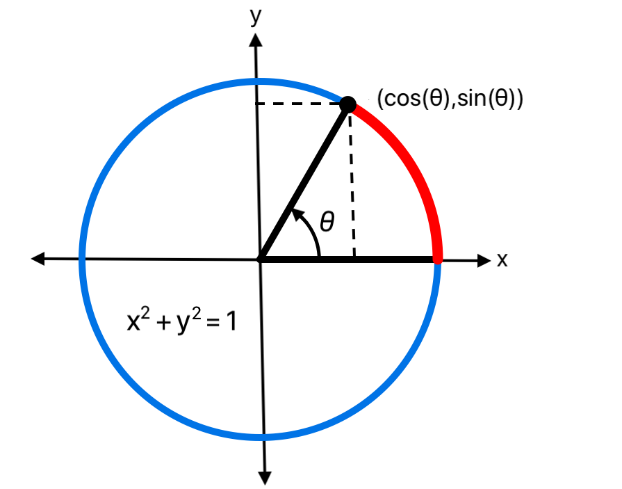
The sine and cosine functions are periodic by definition, as the coordinates on the unit circle determined by the angle θ:
Signals with period 1 are defined with the unit functions defined on the unit interval [0,1), extended to the whole real line using the decimal part of their argument. The decimal part of a number t is the remainder when dividing t by 1, mapping the number t into the unit interval [0,1), computed in Swift with the function truncatingRemainder:
let p = t.truncatingRemainder(dividingBy: 1)
For example:
var t = Double.pi

print("t = \(t)")

var p = t.truncatingRemainder(dividingBy: 1)

print("p = \(p)")

t = t + 1

print("t + 1 = \(t)")

p = t.truncatingRemainder(dividingBy: 1)

print("p = \(p)")
This logs:
t = 3.141592653589793
p = 0.14159265358979312
t + 1 = 4.141592653589793
p = 0.14159265358979312
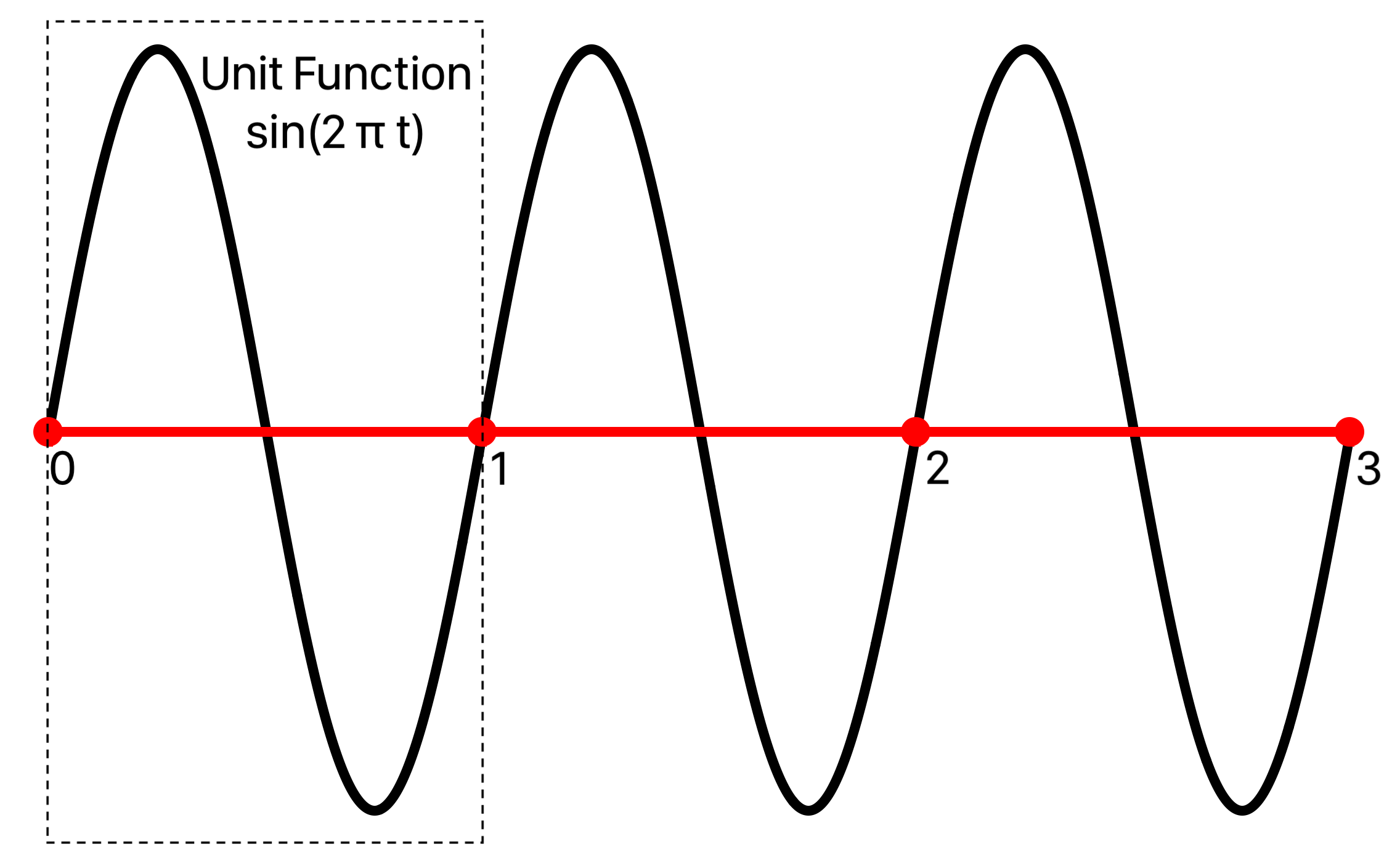
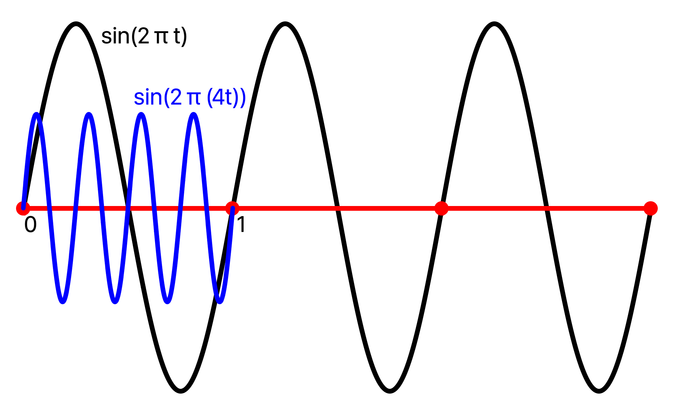
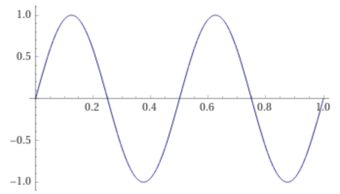
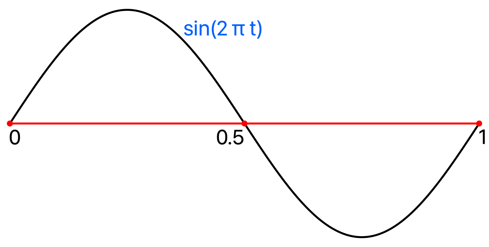
A unit function s(t) defined on [0,1) is evaluated for any t with s(t) = s(t.truncatingRemainder(dividingBy: 1), placing copies of the unit function along the real line. The unit function s(t) = sin(2 π t) is drawn this way here with two copies:
Angular vs. Oscillatory Frequency
The measure θ of an angle is defined to be the arc length a it subtends on the unit circle, θ = a:
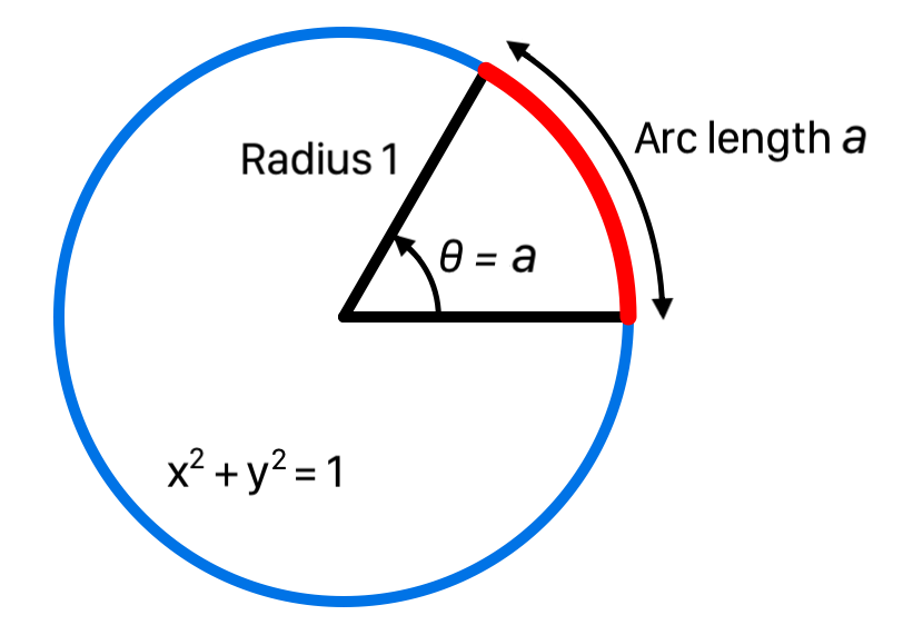
The unit of measure for angles is the radian, which is the angle that subtends an arc length of 1 on the unit circle, denoted by rad.
For a circle with radius r the total arc length C of its circumference is given by C = 2πr. Thus C = 2π for the unit circle, and a radian is the fraction 1/(2π) of its circumference C. A radian subtends the same fraction 1/(2π) of the circumference C of any other circle. But r = C/(2π), so a radian subtends an arc length r on a circle with radius r, hence the name radian.
Frequency is then defined in either oscillatory or angular units:
• Oscillatory frequency f is cycles per second, labelled hertz or Hz. For a periodic function with period k, oscillatory frequency f is f = 1/k, the number of periods in the unit interval [0,1].
• Angular frequency ω is the corresponding radians per second given by ω = 2πf, so 1 Hz (1 cycle per second) corresponds to 1 full angular revolution, or 2π radians per second.
The unit functions have oscillatory frequency of 1 Hz by definition. Signals with other oscillatory frequencies, or periods, are generated with the unit functions by scaling time.
Time Scaling Example
A unit function s(t) can be composed with a time varying function x(t) to obtain a new function s(x(t)) that has period k, for any k. This function is x(t) = t/k, for some constant k, then g(t) = s(x(t)) = s(t/k) is a function with period k, as seen here using the unit periodicity of s:
g(t + k) = s((t + k) / k) = s(t/k + 1) = s(t/k) = g(t).
For example, to generate a signal with 4 Hz, scale time by 4:
Tone Generation
In physics sound is the mechanical vibrations of air that can induce electric signals in devices such as a microphone. The voltage of the electric signal can then be quantized into amplitudes, by sampling over time with an analog-to-digital converter and stored as an array of sample values in a digital audio or video media file.
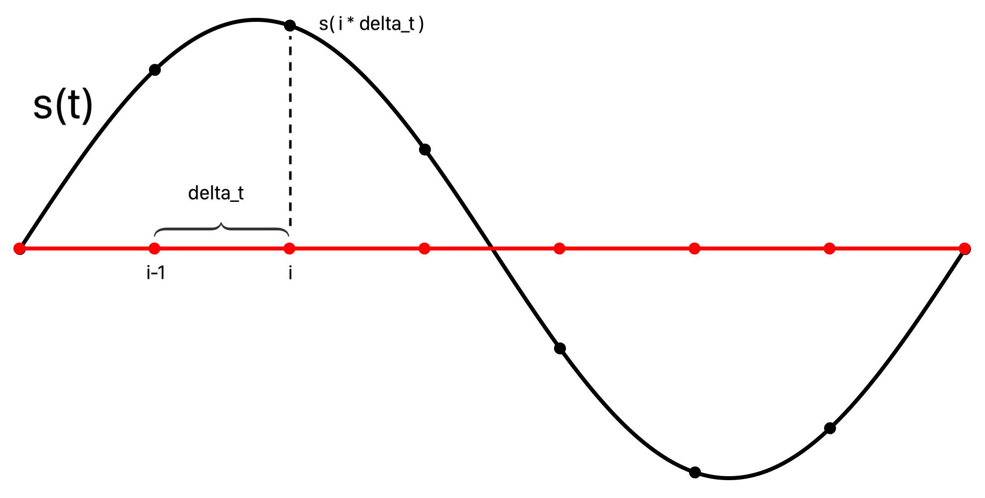
Sound can also be generated from samples using mathematical functions that model physical sources. An idealized pure tone can be modeled by sampling a periodic function s(t) and played using AVAudioEngine. This means that s(t) is evaluated on an indexed grid of enough incremental time intervals, with increments of size delta_t determined by the sampleRate, to fill an audio buffer of a size requested by AVAudioEngine in the AVAudioSourceNodeRenderBlock of the AVAudioSourceNode.
let delta_t:Double = 1.0 / Double(sampleRate)
In this application the sample rate is provided by AVAudioEngine at the time it is set up:
let output = engine.outputNode
let outputFormat = output.inputFormat(forBus: 0)
sampleRate = Float(outputFormat.sampleRate)

print("The audio engine sample rate is \(sampleRate)")
This printed:
"The audio engine sample rate is 44100.0"
When AVAudioEngine is set up an AVAudioSourceNode named srcNode is created with an AVAudioSourceNodeRenderBlock, a function that is called repeatedly to request audio sample buffers for playing. In this block the number of samples requested named frameCount is provided, which along with the cumulative sample count named currentIndex determines the sampleRange, a range of indices ClosedRange<Int> for the grid’s array of samples.
let sampleRange = currentIndex...currentIndex+Int(frameCount-1)
The sample range sampleRange for the current audio buffer is passed to a function audioSamplesForRange where it is iterated to compute the sample times at which to evaluate signal s(t).
for i in sampleRange.lowerBound...sampleRange.upperBound {

    let t = Double(i) * delta_t

    // ... evaluate s(t)
}
audioSamplesForRange returns the samples as an array [Int16] that are then added as Float to the AudioBuffer provided by the AVAudioSourceNodeRenderBlock.
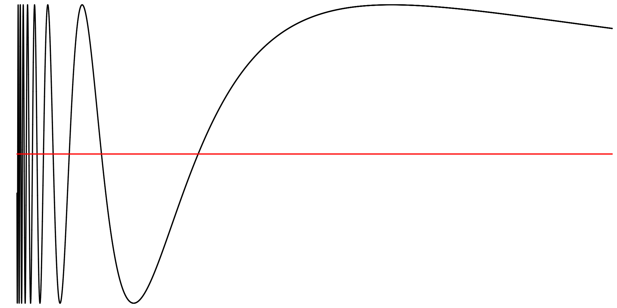
The high sample rate required for audio is due to the classical Nyquist-Shannon sampling theorem which says that a band-limited signal with maximum frequency B can be exactly reconstructed from samples if the sample rate R is twice the maximum frequency B, or R = 2B. Otherwise aliasing occurs, and the reconstructed signal misrepresents the original. Consequently for your hearing range up to 20,000 cycles per second (20kHz) a sample rate greater than 2 x 20,000 = 40,000 samples per second is required. In practice, the sample rate should be chosen strictly greater than twice the maximum frequency B, or R > 2B.
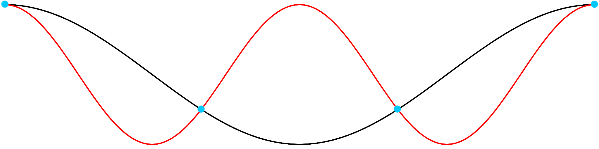
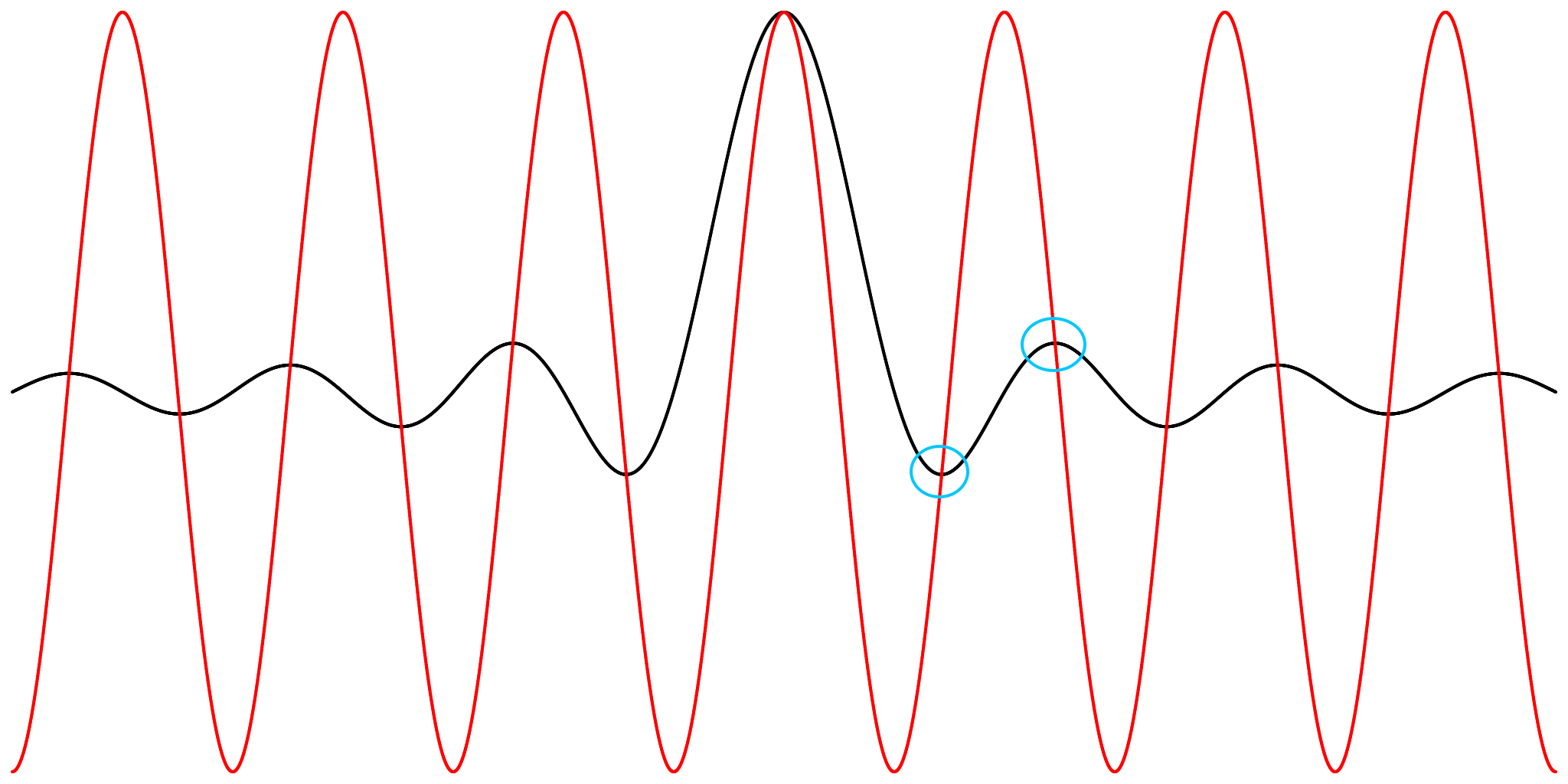
The Fourier transform determines the frequency components of a signal to find the maximum frequency B. If B does not exist, the signal has unlimited frequency components and aliasing occurs for any sample rate. Illustrated here is a higher frequency red signal, which always exists when there is no highest frequency, that is undersampled for a sample rate sufficient for the lower frequency black signal. The blue dot samples are the same for each but miss details of the red signal, causing the red signal to be aliased and indistinguishable from the black signal:
Instantaneous Frequency
Frequency can be time dependent, or variable, by composing a constant frequency signal s(t) of 1 Hz with a time scaling function x(t). The derivative v(t) = dx(t)/dt is the instantaneous rate of change of x(t), or instantaneous frequency. Also x(t) is given by integration of v: x(t) = ∫ v(t). The antiderivative x(t) can be interpreted as a distance traversed at time t in units of the period 1 of s(t), and v(t) as the speed traversing those periods.
In this way a signal s(x(t)) with specific variable frequency can be created by defining v(t) appropriately. As AVAudioEngine requests sample buffers to play and the frequency slider changes, the argument x(t) for the current signal s(t) is updated for smooth play. This is achieved by defining the x(t) as the integral of an instantaneous frequency function v(t) that linearly interpolates the frequency values at the start and end times of the current sample buffer. This means that v(t) = dx/dt, the derivative of x(t), is a frequency ramp.
Previously, in the Time Scaling Example a signal g was defined as:
g(t) = s(x(t)) = s(t/k)
Let f = 1/k, and x(t) = f t, then the rate of change of x is the constant frequency f:
dx(t)/dt = f
and
g(t) = s(x(t)) = s(f t)
Conversely when the rate of change v is a constant f, then x(t) is a linear function f * t + p, for any constant p:
x(t) = ∫ v(t) = ∫ f = f * t + p
For example applying this to the unit function sin(2 π t) with p = 0, the substitution yields sin(2 π f t), the sine wave with constant frequency f Hz.
Constant vs Variable Frequency
The instantaneous rate of change v(t) = dx(t)/dt is illustrated for constant and variable speed to see how the resulting argument x(t) affects the waveform and remaps the periods of the unit function sin(2 π t) with period 1.
Two cases are considered:
1. Constant Instantaneous Frequency
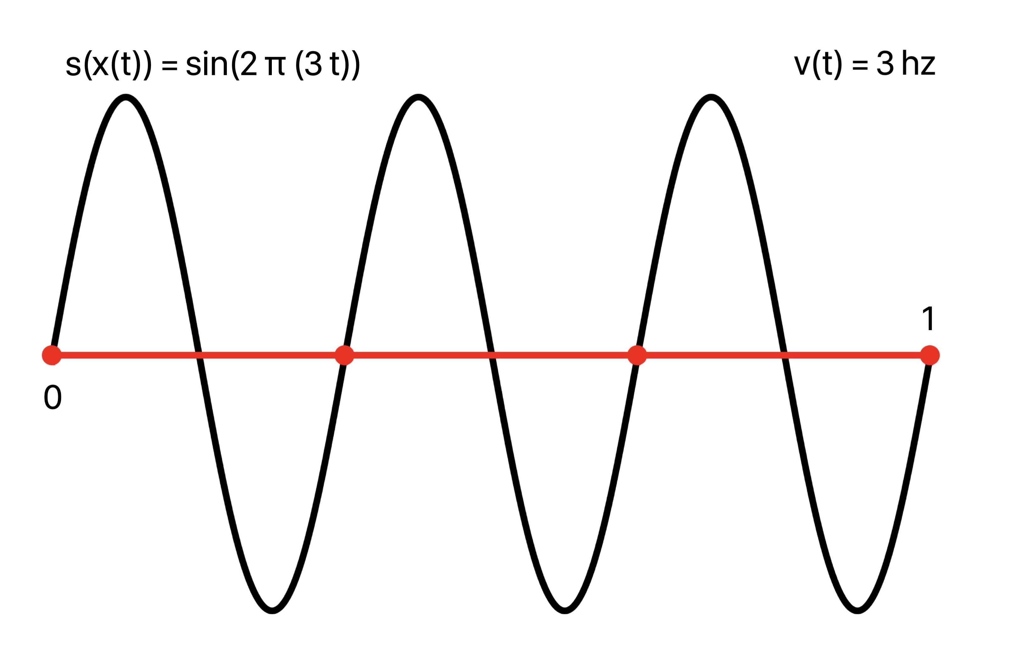
In the case of constant speed 3, v(t) = 3, the periods of sin(2 π t) are traversed at the rate of 3 periods per second, or a constant frequency of 3. This is observed in the composed plot sin(2 π x(t)) = sin(2 π (3 t)) with uniformly spaced crests as time goes on.
The instantaneous frequency is v(t) = 3, with argument given by the antiderivative x(t) = 3 t:
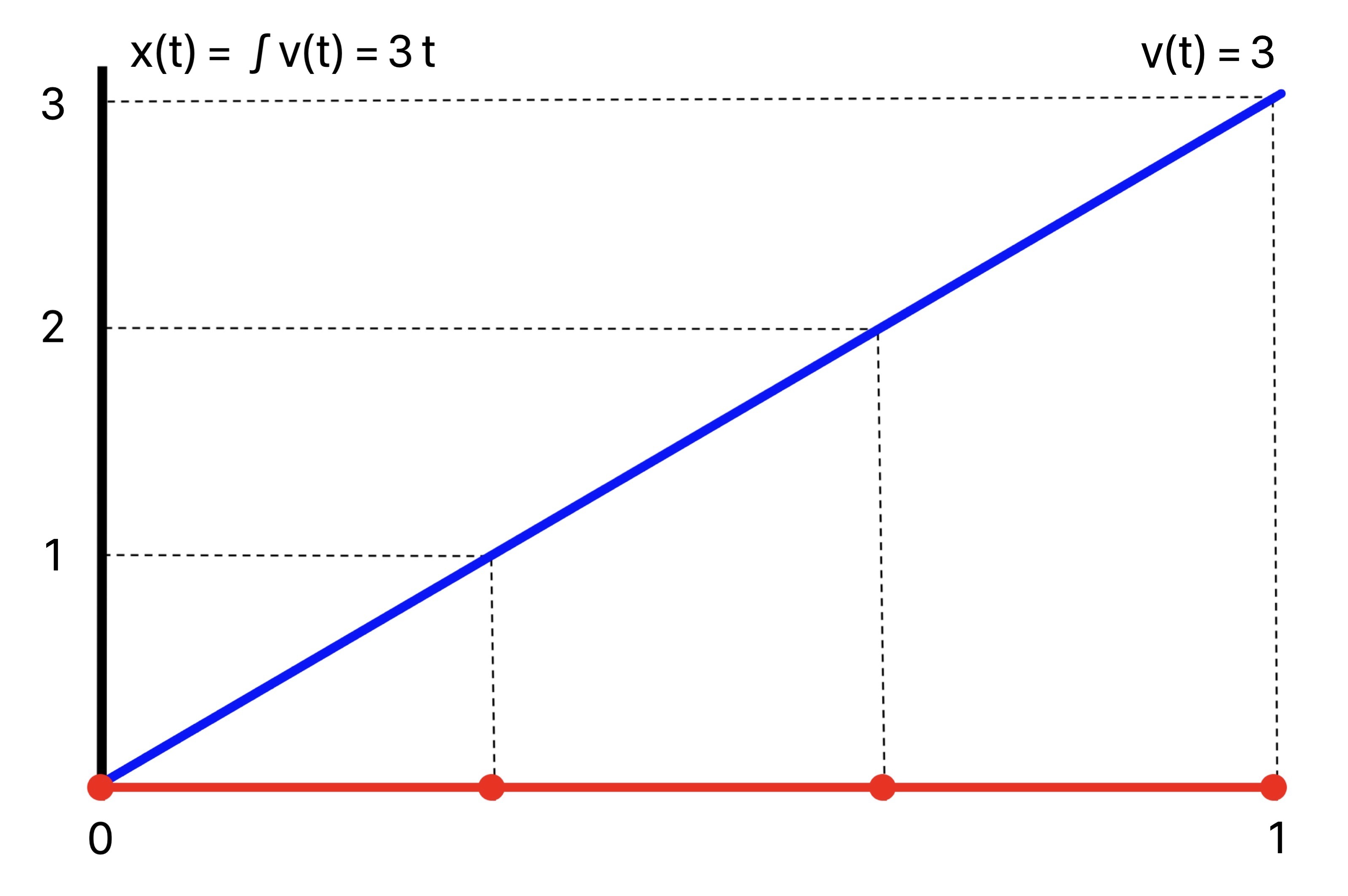
Composing the unit sine wave sin(2 π t) with this argument, plot of sin(2 π (3 t)):
2. Variable Instantaneous Frequency
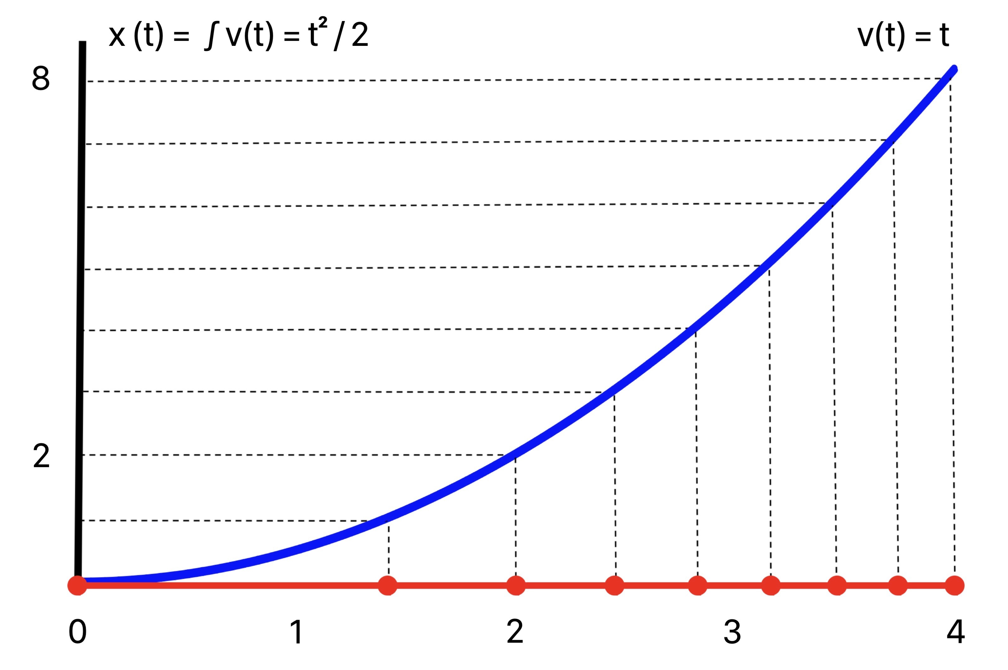
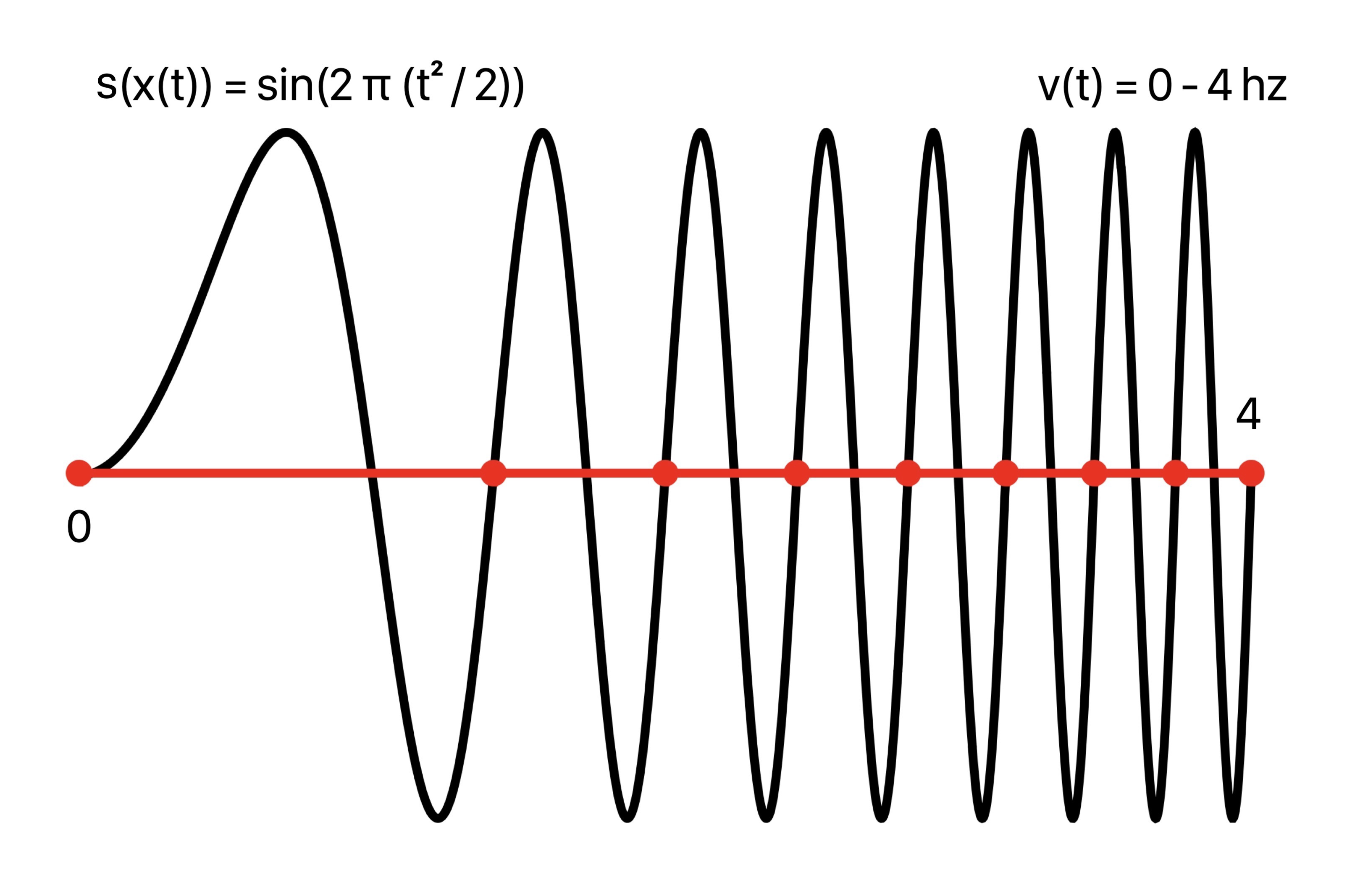
On the other hand, for variable speed proportional to t, v(t) = t, the periods of sin(2 π t) are traversed at an increasing rate, or increasing frequency. This is seen in the composed plot sin(2 π x(t)) = sin(2 π (t^2 / 2)) with more closely spaced crests as time goes on.
The instantaneous frequency is v(t) = t, with argument given by the antiderivative x(t) = t^2 / 2:
Composing the unit sine wave sin(2 π t) with this argument, plot of sin(2 π (t^2 / 2)):
Frequency Ramp
The discussion of Instantaneous Frequency stated a signal s(x(t)) with specific variable frequency can be created by specifying the rate of change function v(t) appropriately, and the argument x(t) is obtained by integration. This is applied here to play the audio for a transition between frequencies when the frequency slider is changed.
When the frequency is changed to v2 the next sample buffer for the current signal s(t) will reflect this change from the previous frequency v1. If the current sample buffer represents an interval of time [t1, t2] then v(t) is derived using linear interpolation to create a ramp between the pair of points (t1, v1) and (t2, v2). Then x(t) = ∫ v(t), and sampling is performed with s(x(t)).
Consider the geometry for this linear interpolation:
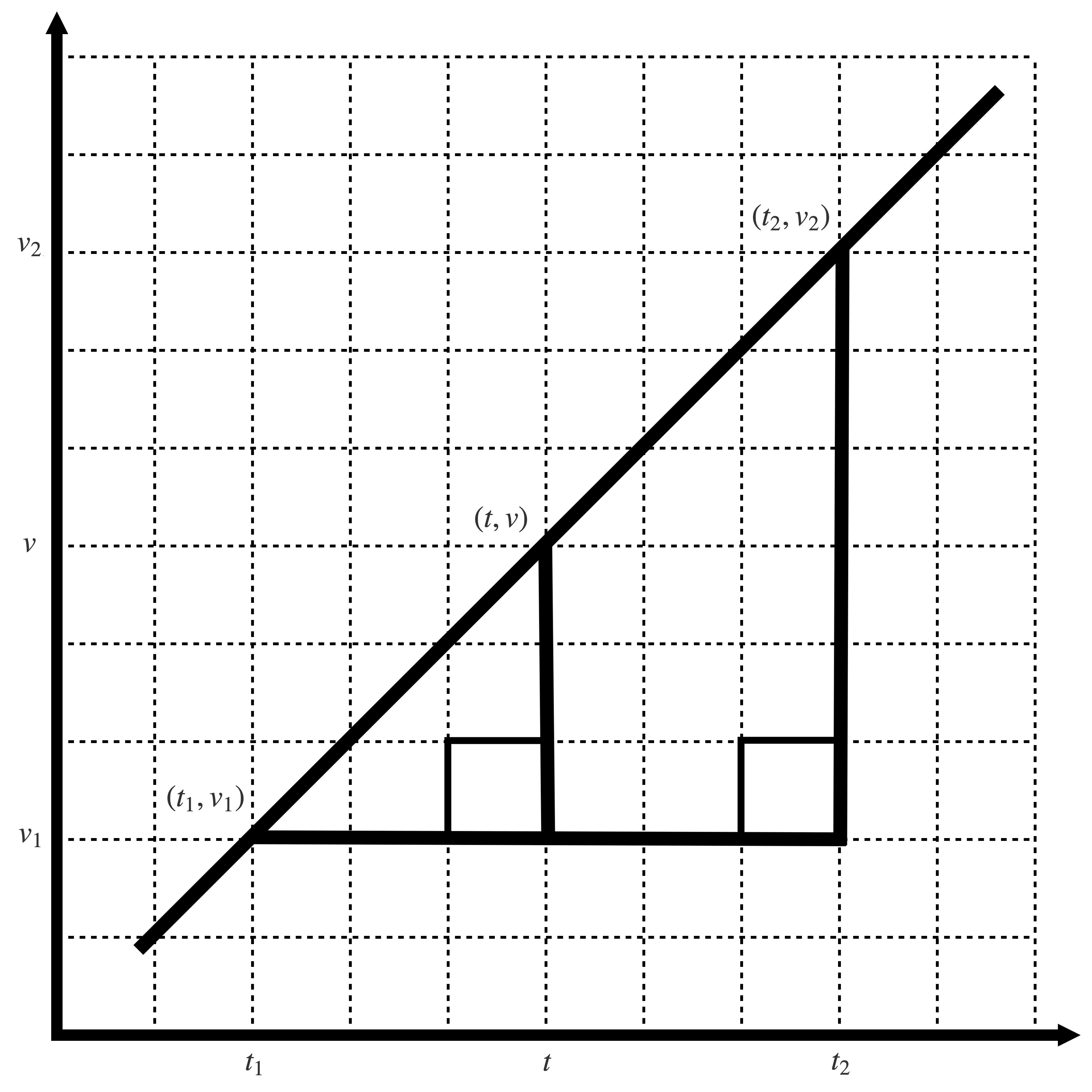
The interpolation relation is given by the similar right triangles:
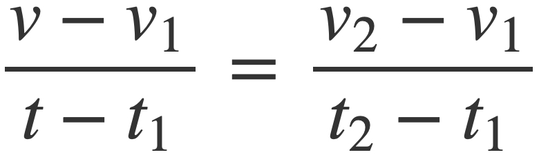
Solving for v(t), or dx/dt, produces the desired frequency ramp:
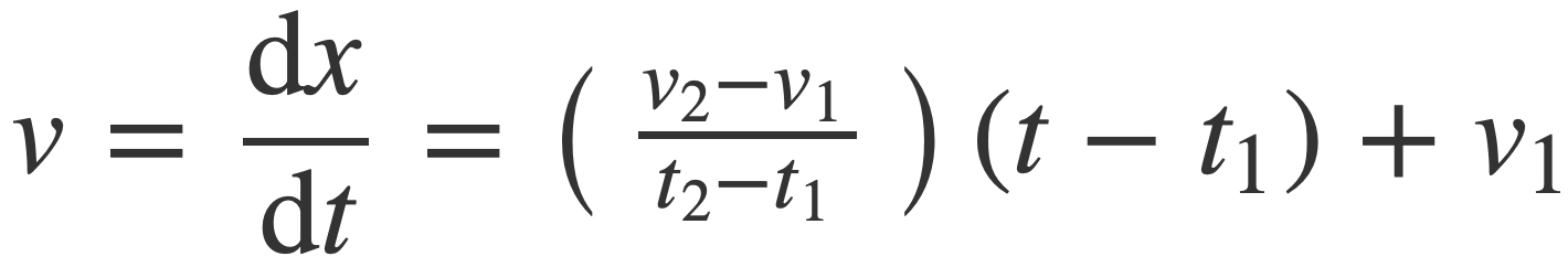
The antiderivative of v, or the signal argument x(t), up to an added constant c is given by:
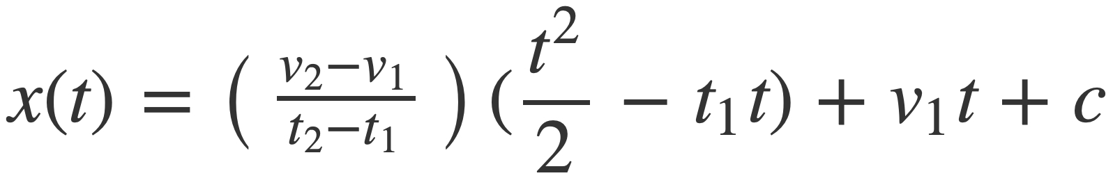
Since the audio signal is invariant under translation c it may be set to zero, and s(x(t) is a function whose frequency changes from v1 to v2 in the time interval [t1,t2].
When v1 = v2 = f, then x(t) = f * t. For the unit function sin(2 π t), substituting f t for t yields the signal sin(2 π f t), which is the familiar form of a sine wave with constant frequency f Hz.
In the general case then sin(2 π x(t)) can be written as sin(2 π g(t) t) when x(t) is factored by pulling out the common factor t:
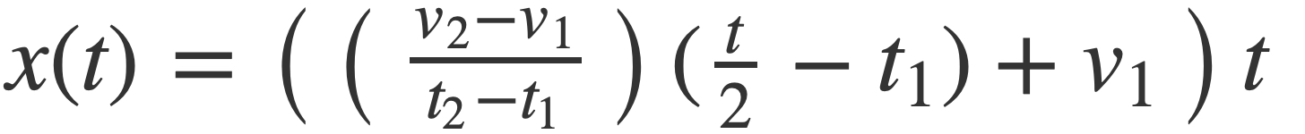
with g(t) given by:
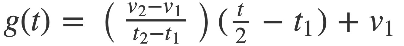
This factorization is useful in the code, where g(t) is implemented in ToneGenerator with the ramp function:
func ramp(_ t:Double, t1:Double, t2:Double, f1:Double, f2:Double) -> Double {
    let df = f2 - f1
    let dt = t2 - t1

    if dt == 0 {
        return f1
    }

    return f1  + (df / dt) * (t / 2 - t1)
}
The ramp function is used in generateRampedSamples to set the frequency of the current Component for sampling.
Example. Using these equations a signal that transitions from 2 to 6 Hz on the time interval [1,2] is given by
sin(2 π g(t) t)
where
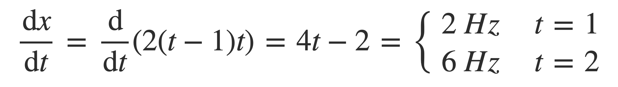
g(t) = 4 (t / 2 - 1) + 2 = 2 (t - 1)
Check:
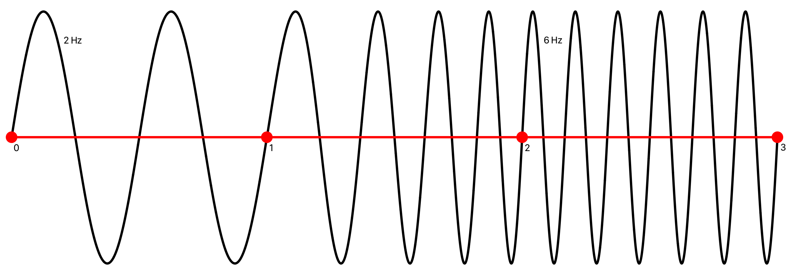
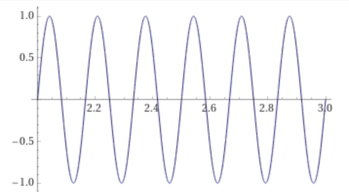
Combining this frequency ramp with a 2 Hz signal sin(2 π 2 t) and a 6 Hz signal sin(2 π 6 t), a piecewise signal is formed:
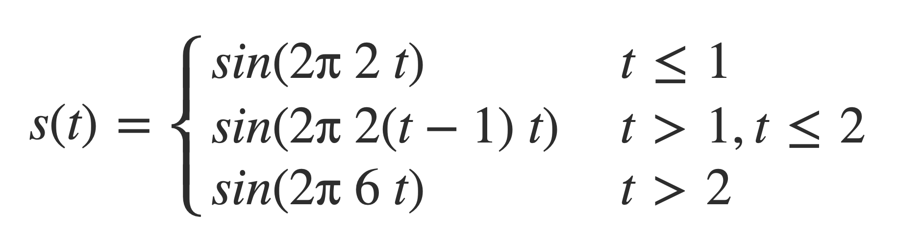
This signal is initially 2 Hz on the interval [0,1], transitions from 2 to 6 Hz on the interval [1,2], and remains 6 Hz on [2,3]:
Plot the parts of the piecewise signal s(t) individually:
plot sin(2 π 2 t) on 0,1
plot sin(2 π 2(t-1) t) on 1,2
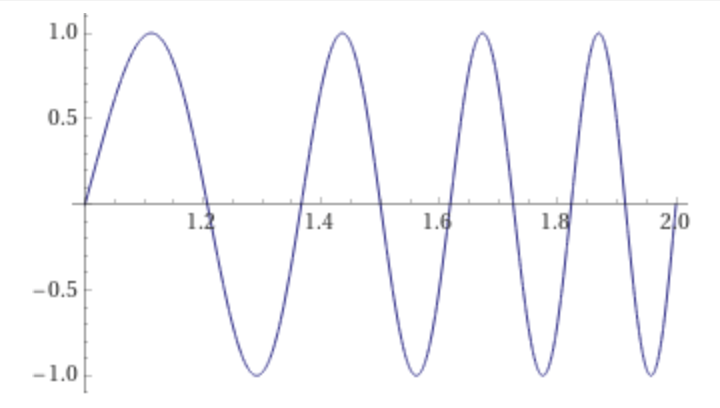
plot sin(2 π 6 t) on 2,3
Although not necessary for this example, piecewise combination of variable frequency signals this way in general requires phase adjustments to remove discontinuities that cause clicking sounds in the audio.
Phase Adjustment
As the instantaneous frequency v(t) is recalculated for each frequency change by the slider, a new argument x(t) is produced that can create a discontinuity between the previous and current composition s(x(t)). Discontinuity can cause clicking sounds in the audio when play advances to the next sample buffer.
The discontinuity can be removed by offsetting the value of the argument of the current signal s by an amount so that the first sample value with the current frequency equals that of the last sample value with the previous frequency.
Example. Constant 2 Hz to constant 4 Hz
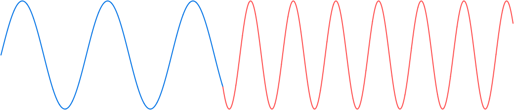
Consider sampling the sine wave on the interval [0,3] when the frequency changes from 2 Hz to 4 Hz at time 1.3. When the samples are plotted in blue prior to the change and red after, a large jump in the values is evident:
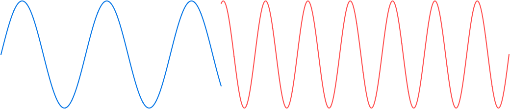
The discontinuity is removed by offsetting the value of the argument of the current signal s, red on the right, by an amount that causes the first sample value with the current frequency to match that of the last sample value with the previous frequency:
Example. Constant 1 Hz to ramp from 1 Hz to 16 Hz
Now consider sampling the sine wave on the interval [0,3] where it has frequency 1 Hz up to time 1.3, and then the frequency changes from 1 Hz to 16 Hz on [1.3,3.0] using a frequency ramp. A large jump in the values is again evident:
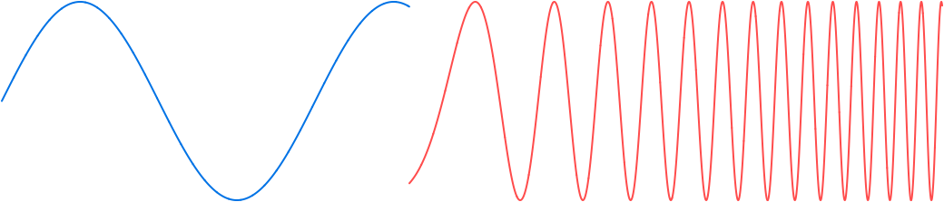
Again, the discontinuity can be mitigated by offsetting the value of the argument of the current signal s on the right:
Compute Accumulating Offsets
Let T be the time of the change in frequency, x1(t) be the argument of the signal s before T, and x2(t) the argument after. The offset, or phase adjustment, is then D = (x1(T) - x2(T)).
This way the sampling signal after T is not s(x2(t)) but s(x2(t) + D).
Check at time T:
s(x2(T) + D) = s(x2(T) + (x1(T) - x2(T))) = s(x1(T)),
removing the discontinuity.
This procedure is used repeatedly when generating samples for any sample buffer, whether or not an actual change in frequency occurs, i.e. for degenerate ramps when v1 equals v2, and no matter the sampling function for the previous buffer.
Moreover, phase adjustment is accumulative. The current phase adjustment is appended by any previous phase adjustment as samples are generated for every successive audio buffer request.
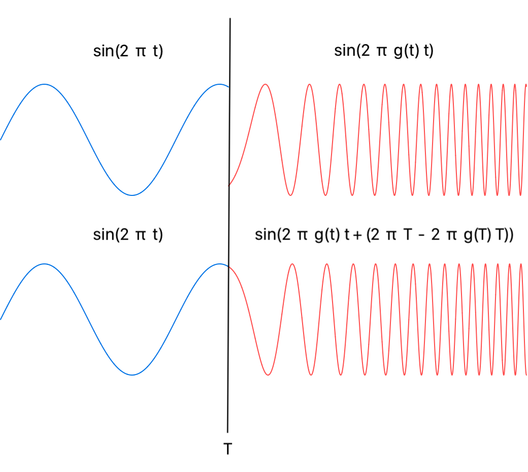
Sine Example
Using a frequency ramp a function g(t) is produced such that when s is composed with g(t) t the samples generate a signal whose frequency changes from v1 to v2 on a given interval [t1,t2].
Let the current signal s be the unit function sin(2 π t), so the composed signal is sin(2 π g(t) t). Suppose the transition with possible discontinuity occurs at time T.
Then instead of sampling the functions sin(2 π t) and sin(2 π g(t) t) before and after the time T, the argument of the composition sin(2 π g(t) t) is offset by the difference D of the respective arguments 2 π t and 2 π g(t) t evaluated at the time of the transition T:
D = (2 π T) - (2 π g(T) T)
Then the sampling function after time T is sin(2 π g(t) t + D) or sin(2 π g(t) t + (2 π T - 2 π g(T) T)).
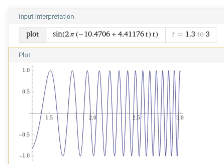
Revisit Example: Constant 1 Hz to ramp from 1 Hz to 16 Hz
The general form of g(t) is:
Substitute v1 = 1, v2 = 16, t1 = 1.3, t2 = 3 into the general form to get:
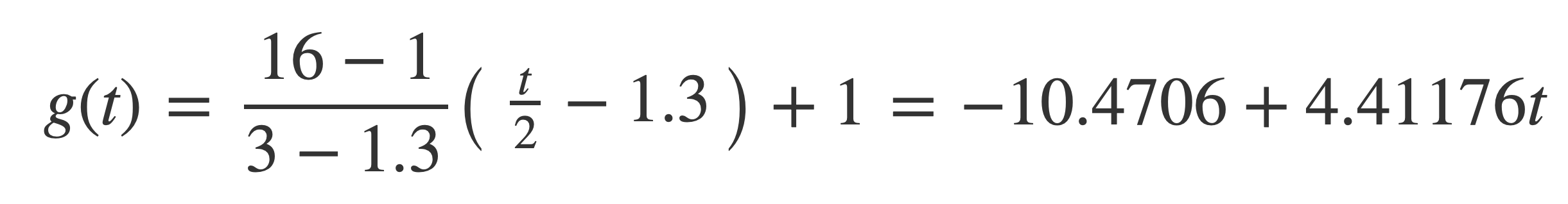
Plot the ramp signal by substituting this expression for g(t) into sin(2 π g(t) t):
plot sin(2 π (-10.4706 + 4.41176 t) t) on 1.3,3.0
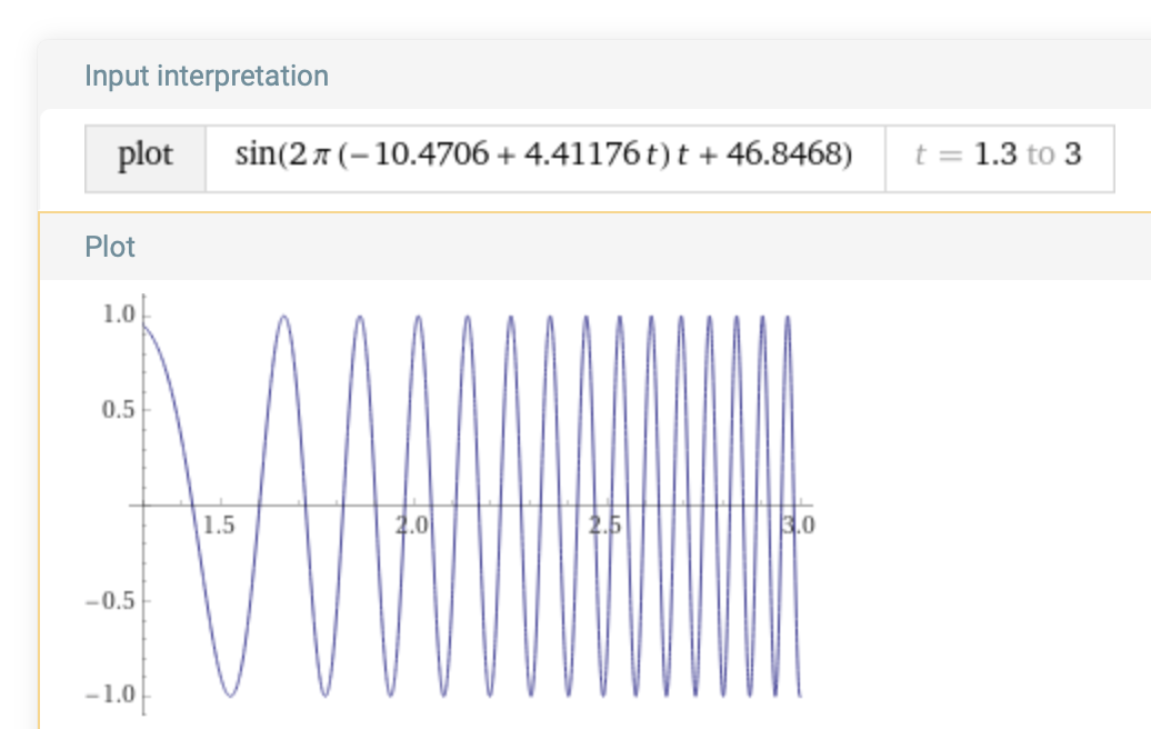
Apply the phase offset at T = 1.3, first calculate D:
D = (2 π T) - (2 π g(T) T) = (2 π 1.3) - (2 π g(1.3) 1.3)
But g(1.3) = -10.4706 + 4.41176 * 1.3 = -4.735312:
D = (2 π 1.3) - (2 π (-4.735312) 1.3) = 46.8468
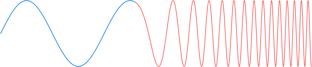
Now plot the ramp signal with the g(t) and the offset D, sin(2 π g(t) t + D):
plot sin(2 π (-10.4706 + 4.41176 t) t + 46.8468) on 1.3,3.0
Compare applying the phase adjustment to fix the transition discontinuity at T = 1.3:
TonePlayer Unit Functions
Unit function types are defined by the WaveFunctionType enumeration, corresponding to unit functions (_ t:Double) -> Double on [0,1] for defining periodic signals with period 1. Signals with other oscillatory frequencies, or periods, are generated with the unit functions by scaling time.
// Note : wavefunctions should have values <= 1.0, otherwise they are clipped in sample generation
// Partial sum value of the Fourier series can exceed 1
enum WaveFunctionType: String, Codable, CaseIterable, Identifiable {
    case sine = "Sine"
    case square = "Square"
    case squareFourier = "Square Fourier"
    case triangle = "Triangle"
    case triangleFourier = "Triangle Fourier"
    case sawtooth = "Sawtooth"
    case sawtoothFourier = "Sawtooth Fourier"
    var id: Self { self }
}
These are the periodic functions sampled to fill audio sample buffers requested by AVAudioEngine, or to generate WAV file with ToneWriter class method saveComponentSamplesToFile.
A tone is defined with a struct Component.
struct Component {
    var type:WaveFunctionType

    var frequency:Double
    var amplitude:Double
    var offset:Double

    func value(x:Double) -> Double {
        return wavefunction(x, frequency, amplitude, offset, type)
    }
}
The unit function for the type is provide by the unitFunction lookup function.
func unitFunction( _ type: WaveFunctionType) -> ((Double)->Double) {

    switch type {
        case .sine:
            return sine(_:)
        case .square:
            return square(_:)
        case .triangle:
            return triangle(_:)
        case .sawtooth:
            return sawtooth(_:)
        case .squareFourier:
            return { t in square_fourier_series(t, fouierSeriesTermCount) }
        case .triangleFourier:
            return { t in triangle_fourier_series(t, fouierSeriesTermCount) }
        case .sawtoothFourier:
            return { t in sawtooth_fourier_series(t, fouierSeriesTermCount) }
    }
}
The value of a component is computed by wavefunction using truncatingRemainder to extend to the positive real line the unit function returned by the unitFunction lookup function.
func wavefunction(_ t:Double, _ frequency:Double, _ amplitude:Double, _ offset:Double, _ type: WaveFunctionType) -> Double {

    let x = frequency * t + offset

    let p = x.truncatingRemainder(dividingBy: 1)

    return amplitude * unitFunction(type)(p)
}
Sine Wave

The wave function type .sine is defined on [0,1] with:
func sine(_ t:Double) -> Double {
    return sin(2 * .pi * t)
}
Square Wave

The wave function type .square is defined on [0,1] with:
func square(_ t:Double) -> Double {
    if t < 0.5 {
        return 1
    }
    return -1
}
Triangle Wave

The wave function type .triangle is defined on [0,1] with:
func triangle(_ t:Double) -> Double {
    if t < 0.25 {
        return 4 * t
    }
    else if t >= 0.25 && t < 0.75 {
        return -4 * t + 2
    }
    return 4 * t - 4
}
Sawtooth Wave

The wave function type .sawtooth is defined on [0,1] with:
func sawtooth(_ t:Double) -> Double {
    return t
}
TonePlayer Fourier series
For each of the signal types square, sawtooth and triangle a partial Fourier series is computed as an alternative signal type. The formula implemented are described in Fourier series at MathWorld using the general form of the Fourier series.
Periodic functions can be expressed as infinite sums of sine and cosine waves using Fourier series. Truncated Fourier series of the unit functions .square, .triangle and .sawtooth are provided for comparison.
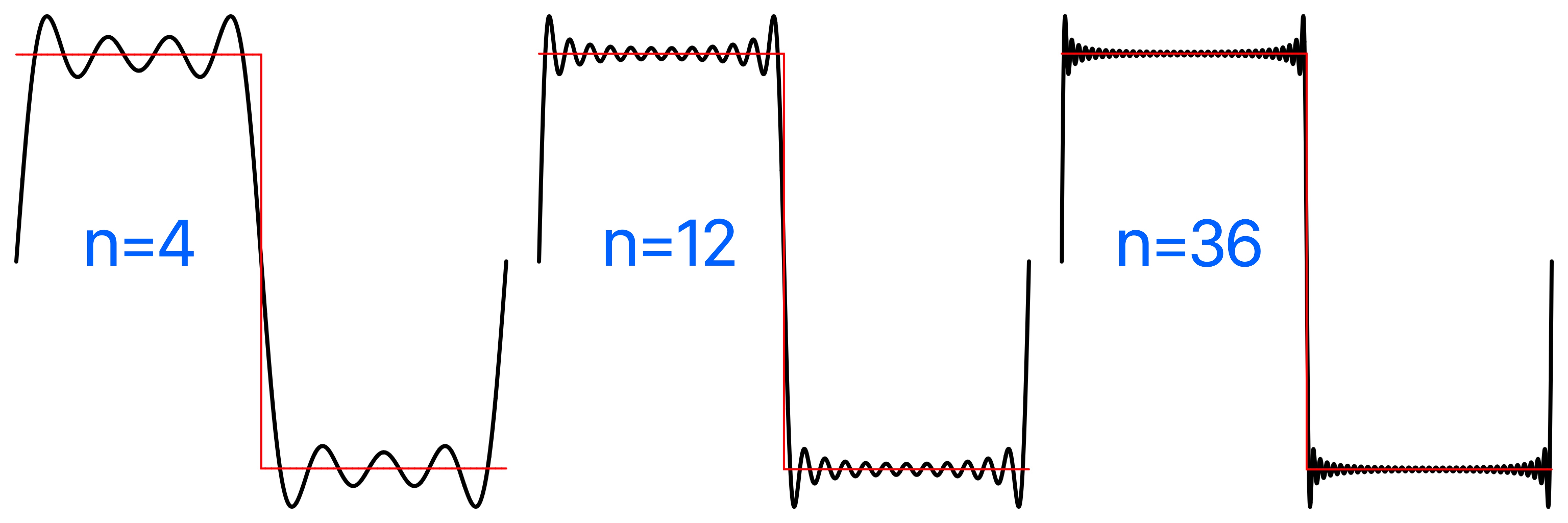
For a differentiable function with discontinuities, such as the square and sawtooth, the Fourier series partial sums converge to the function at points where it is differentiable, but always exhibit significant approximation error near any discontinuity, referred to as Gibbs phenomenon.
In the implementation wave functions should have values ≤ 1.0 as they are converted to Int16 values, but the partial sums of the Fourier series can exceed 1. Values > 1 are clipped during sampling since Int16 audio samples are bounded to the range Int16.min...Int16.max = -32768...32767.
Square Fourier
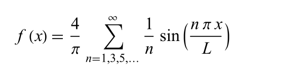
See Square Wave Fourier series for a derivation of this formula, with L=½ for the Square unit function.
square_fourier_series implements this formula where n is the desired number of terms.
func square_fourier_series(_ t:Double, _ n:Int) -> Double {

    var sum = 0.0

    for i in stride(from: 1, through: n * 2, by: 2) {
        let a = Double(i)
        sum += ((1.0 / a) * sin(2 * a * .pi * t))
    }

    return (4.0 / .pi) * sum
}
Plot of the square Fourier series comparatively using square_fourier_series, the square wave plotted in red, the Fourier series in black. For a differentiable function with discontinuities, such as the square and sawtooth, the Fourier series partial sums converge to the function at points where it is differentiable, but always exhibit significant approximation error near the discontinuity, referred to as Gibbs phenomenon.
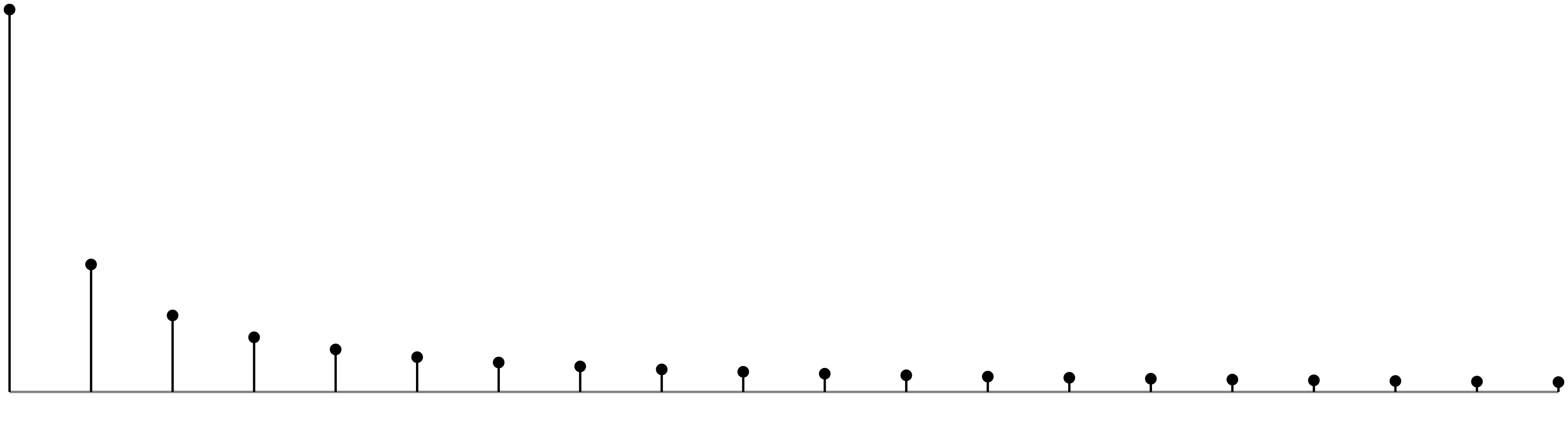
Square Wave Fourier Coefficients:
Triangle Fourier
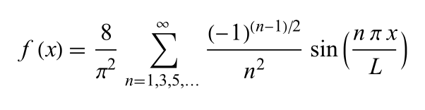
See Triangle Wave Fourier series for a derivation of this formula, with L=½ for the Triangle unit function.
triangle_fourier_series implements this formula where n is the desired number of terms.
func triangle_fourier_series(_ t:Double, _ n:Int) -> Double {

    var sum = 0.0

    for i in stride(from: 1, through: n, by: 2) {
        let a = Double(i)
        sum += ((pow(-1,(a-1)/2) / pow(a, 2.0)) * sin(2 * a * .pi * t))
    }

    return (8.0 / pow(.pi, 2.0)) * sum
}
Plot of the triangle Fourier series comparatively using triangle_fourier_series, the triangle wave plotted in red, the Fourier series in black.
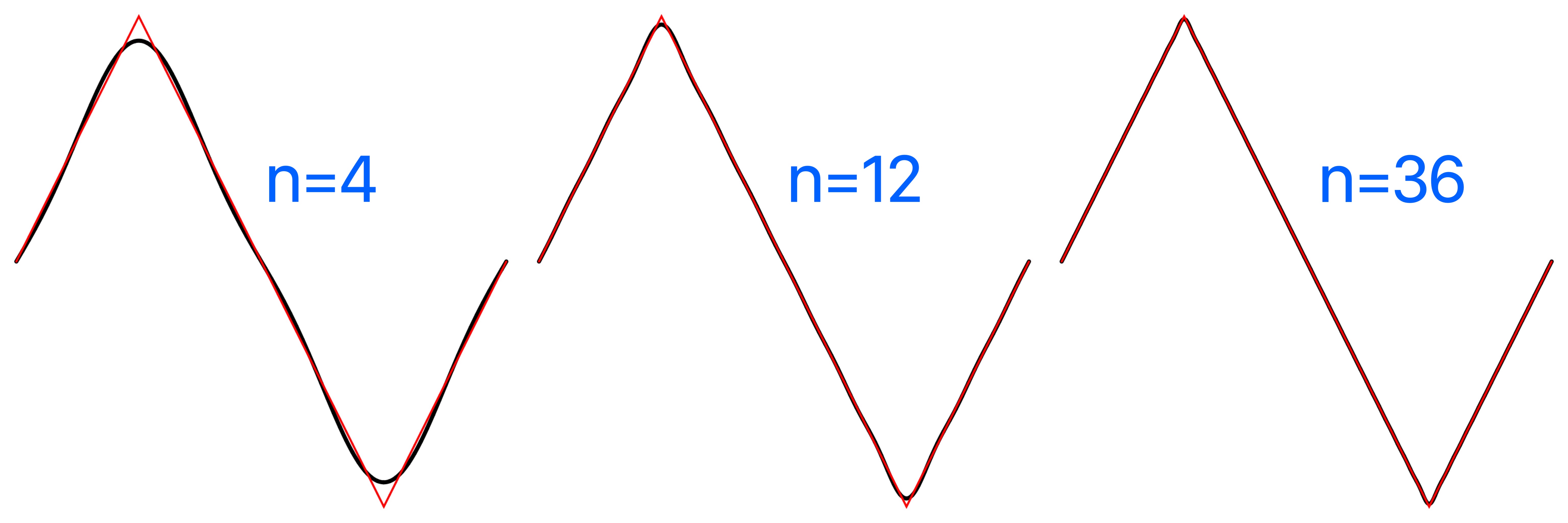
Triangle Wave Fourier Coefficients:
Sawtooth Fourier
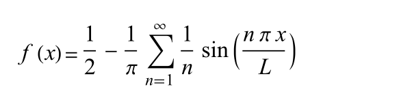
See Sawtooth Wave Fourier series for a derivation of this formula, with L=½ for the Sawtooth unit function.
sawtooth_fourier_series implements this formula where n is the desired number of terms.
func sawtooth_fourier_series(_ t:Double, _ n:Int) -> Double {

    var sum = 0.0

    for i in 1...n {
        sum += sin(Double(i) * 2.0 * .pi * t) / Double(i)
    }

    return 0.5 + (-1.0 / .pi) * sum
}
Plot of the sawtooth Fourier series comparatively using sawtooth_fourier_series, the sawtooth wave plotted in red, the Fourier series in black. For a differentiable function with discontinuities, such as the square and sawtooth, the Fourier series partial sums converge to the function at points where it is differentiable, but always exhibit significant approximation error near the discontinuity, referred to as Gibbs phenomenon.
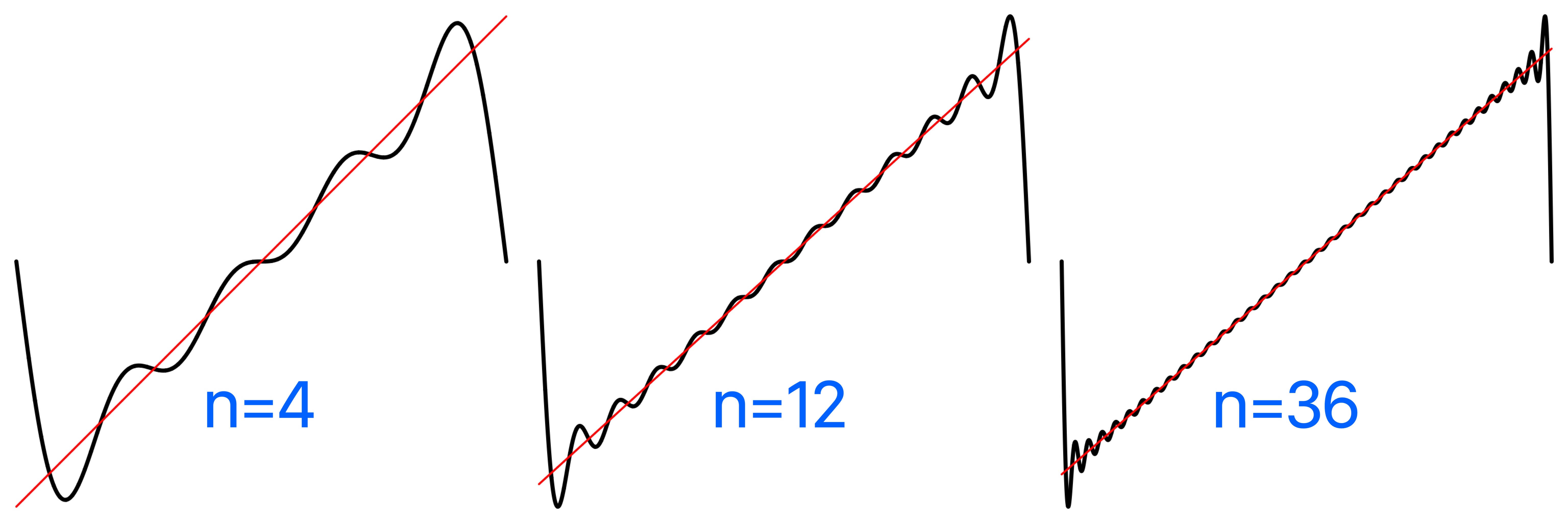
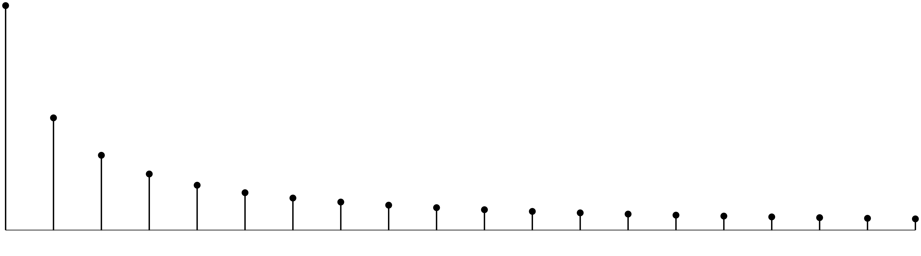
Sawtooth Wave Fourier Coefficients:
Writing Tone Files
A tone defined by a Component can be written to a WAV file of specified duration with the ToneWriter class method toneWriter.saveComponentSamplesToFile that uses AVFoundation to write audio sample buffers.
var toneWriter = ToneWriter()

func TestToneWriter(wavetype: WaveFunctionType, frequency:Double, amplitude: Double, duration: Double, scale: ((Double)->Double)? = nil) {
    if let documentsURL = FileManager.documentsURL(filename: nil, subdirectoryName: nil) {
        print(documentsURL)

        let destinationURL = documentsURL.appendingPathComponent("tonewriter - \(wavetype), \(frequency) hz, \(duration).wav")

        toneWriter.scale = scale

        toneWriter.saveComponentSamplesToFile(component: Component(type: wavetype, frequency: frequency, amplitude: amplitude, offset: 0), duration: duration,  destinationURL: destinationURL) { resultURL, message in
            if let resultURL = resultURL {
#if os(macOS)
                NSWorkspace.shared.open(resultURL)
#endif
                let asset = AVAsset(url: resultURL)
                Task {
                    do {
                        let duration = try await asset.load(.duration)
                        print("ToneWriter : audio duration = \(duration.seconds)")
                    }
                    catch {
                        print("\(error)")
                    }
                }
            }
            else {
                print("An error occurred : \(message ?? "No error message available.")")
            }
        }
    }
}
In GenerateTonePlayerSample the ToneWriter is used to create the audio file sample for the model signal in the energy spectral density computation.
The duration is calculated for the time at which the signal has decayed to effectively zero:
/*
 Solve for t: e^(-2t) = 1/Int16.max, smallest positive value of Int16 (where positive means > 0)
 */
func GenerateTonePlayerSample() {
    let D = -log(1.0/Double(Int16.max)) / 2.0 // D = 5.198588595177692
    print(D)
    let scale:((Double)->Double) = {t in exp(-2 * t)}
    TestToneWriter(wavetype: .sine, frequency: 440, amplitude: 1, duration: D, scale: scale)
}
Fourier Analysis
A pure audio tone of a single oscillatory frequency f Hz is produced with the function sin(2πft). In contrast, a model signal with a continuum of frequencies is produced by multiplying sin(2πft) by the function e-αt and the Heaviside step function to simulate a pulse vibration decaying at rate α.
To see this the Fourier transform is applied to find a frequency description that provides the weights of the signals frequency components e-iωt.
Additionally, plots with contrasting values of the decay rate α reveal the energy spectral density is less concentrated in the frequency domain when the signal is more concentrated in the time domain.
The Fourier transform integrals do not exist in the usual sense for some signals, such as the idealized constant and periodic signals. The Delta Function is defined to extend applicability of the Fourier transform to these cases.
Fourier transform
The Fourier transform for non-periodic functions is introduced and compared to the complex version of the Fourier series for periodic functions. The form of the Fourier transform varies and a particular form is chosen for the rest of the discussion. The Fourier transform is used later in the derivation of the reconstruction formula of the Nyquist-Shannon sampling theorem.
Complex Fourier series for Periodic Functions
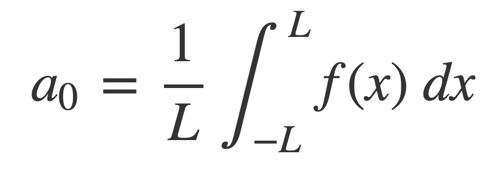
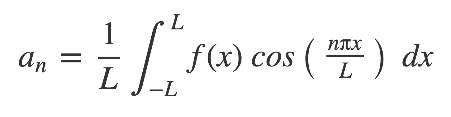
Fourier series at MathWorld provides the expression of a periodic function f(x), periodic on [-L,L], as a weighted infinite sum of trigonometric functions sin and cos over a discrete set of frequencies:
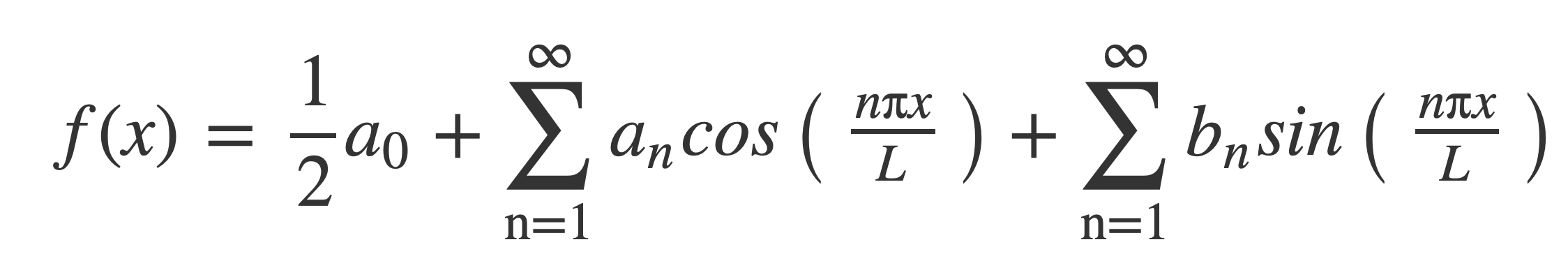
With coefficients given by:
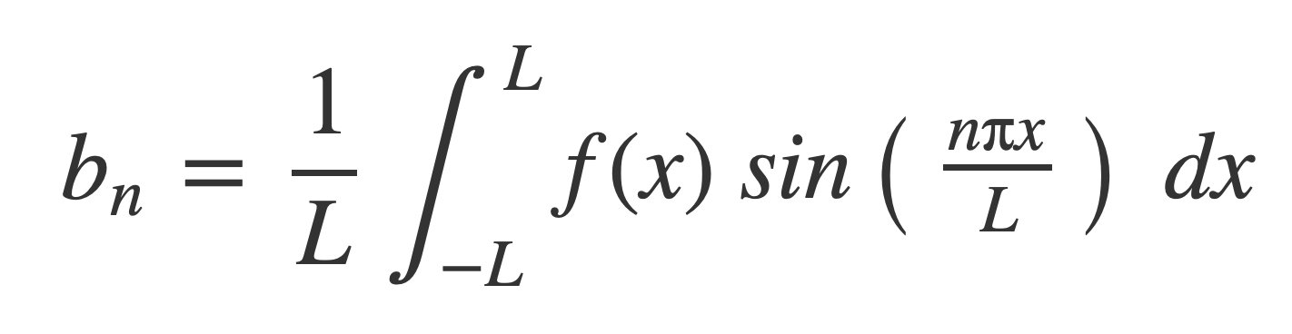
For any k the limits of integration can be changed from -L,L to k,k+2L when evaluating the coefficients a0, an and bn. k is set to 0 in the calculations of the Square Fourier, Triangle Fourier and Sawtooth Fourier in TonePlayer Fourier series.
Euler’s Formula connects the trigonometric functions to the complex exponential function:
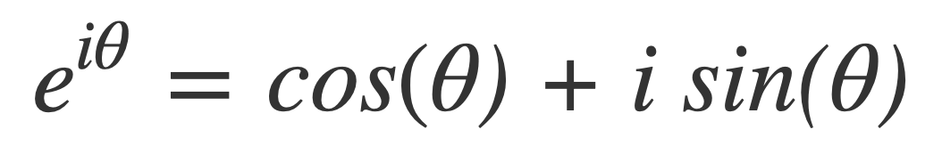
Where i is the imaginary unit : i2 = −1
The trigonometric functions can be expressed in terms of the complex exponential function:
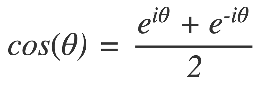
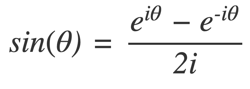
With Euler’s Formula the Fourier series of a function can be expressed using the complex exponential function as a sum of weighted frequency components of the form ei2πfx, where f is oscillatory frequency.
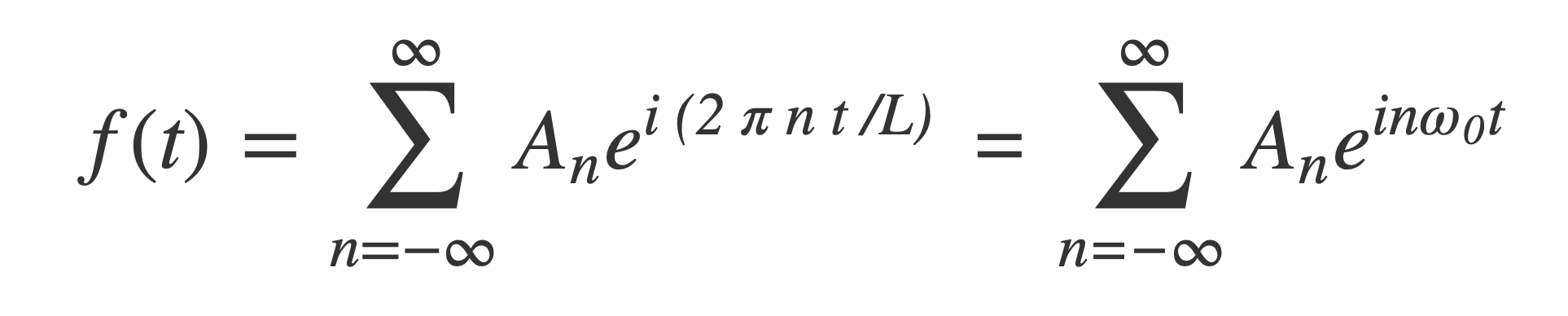
For a function periodic in [-L/2,L/2] the complex Fourier series is:
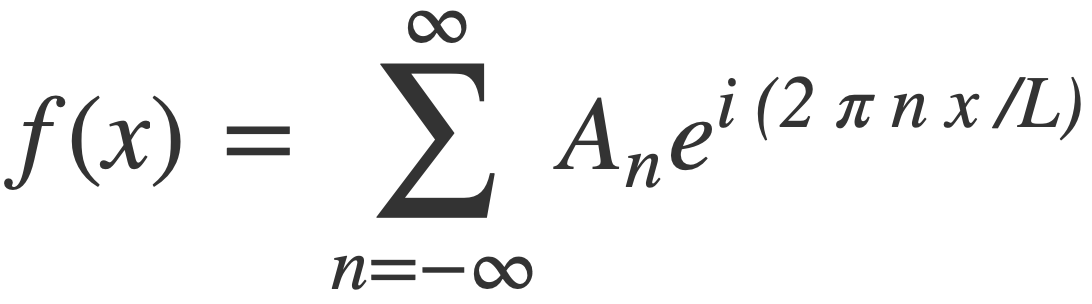
Each frequency component is a multiple n of the fundamental frequency 1/L of f(x), with weight An given by:
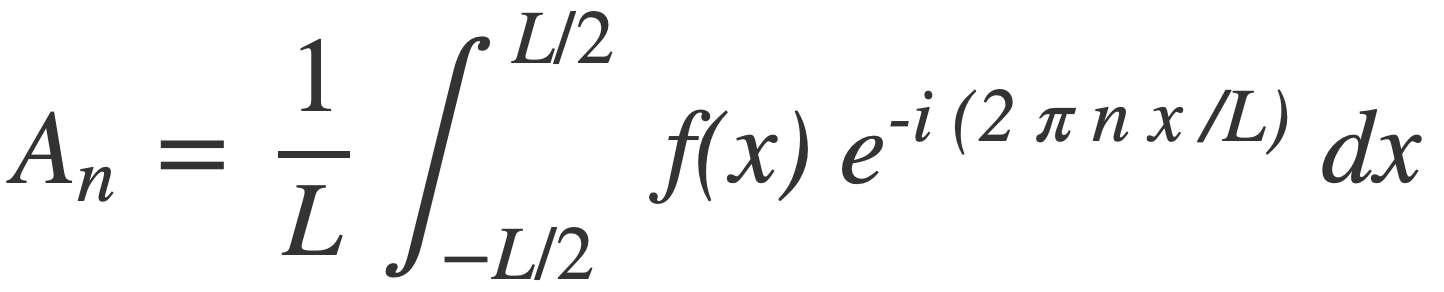
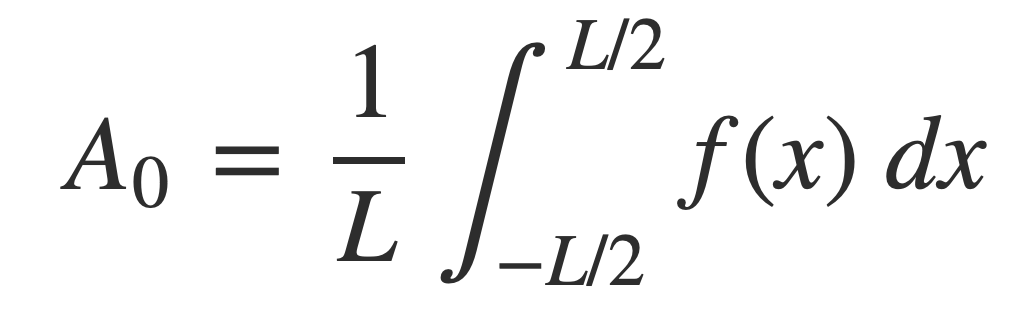
A0, the non-oscillatory or zero frequency DC component, is the average value of the signal over its period, given by:
The conversion of the trigonometric form to this complex form is described in Fourier series at MathWorld.
The complex Fourier series will be used to derive the reconstruction formula of the Nyquist-Shannon sampling theorem.
Convergence of Fourier series
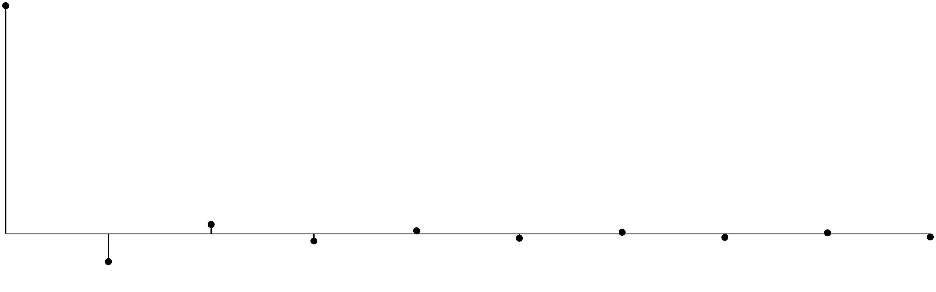
Pointwise convergence of Fourier series means that the complex Fourier series representation of f holds for all x:
Pointwise convergence at x occurs if f is differentiable at x. If there is a jump discontinuity at x, but the left and right side derivatives exist, then it converges to the average of the left and right side limits of f. At discontinuities every partial sum of the Fourier series has a significant approximation error near the discontinuity, referred to as Gibbs phenomenon.
The square wave plotted in red, the Fourier series in black, various number of terms n.
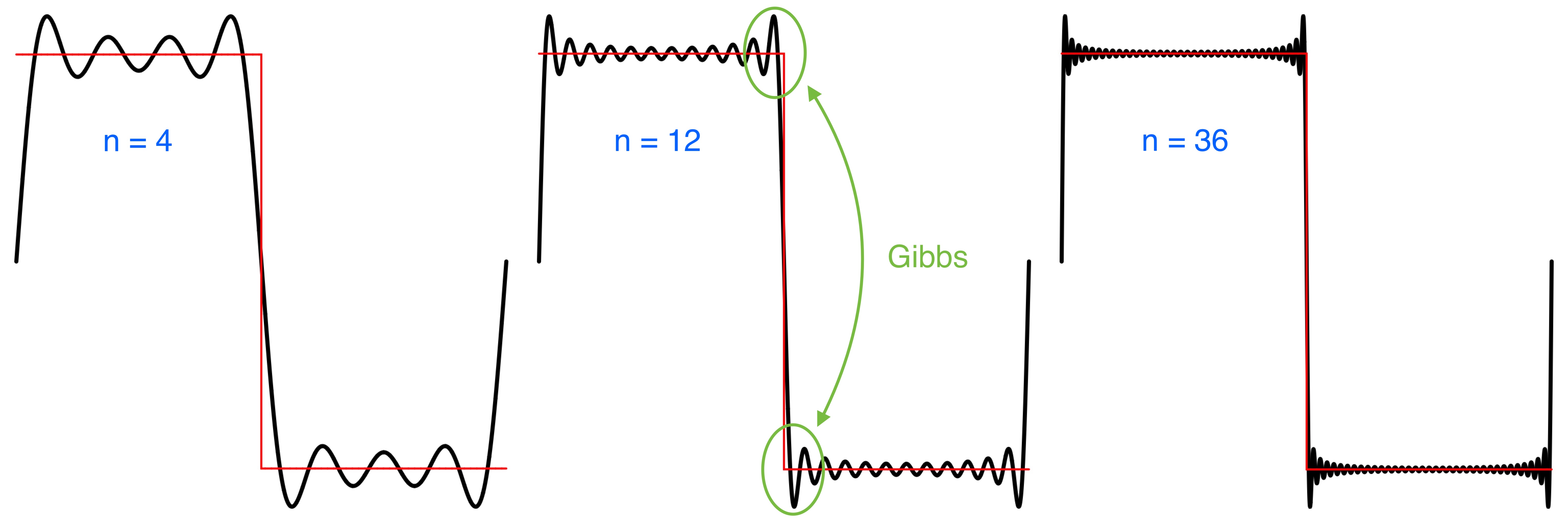
See TonePlayer Fourier series where the Fourier series of the discontinuous square and sawtooth functions are given.
Fourier transform for Non-Periodic Functions
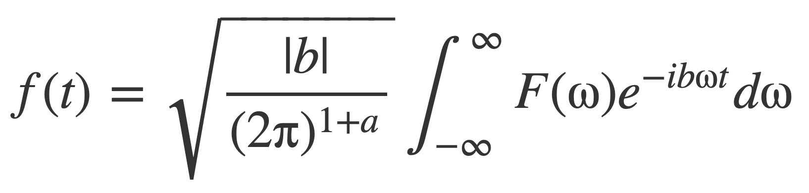
The inverse Fourier transform of non-periodic functions is the analogue of the complex Fourier series for periodic functions:
![]()
It expresses a non-periodic function f(t) as an improper integral over a continuum of weighted frequency components e-iωt, where ω is angular frequency, and values of F(ω) are the weights
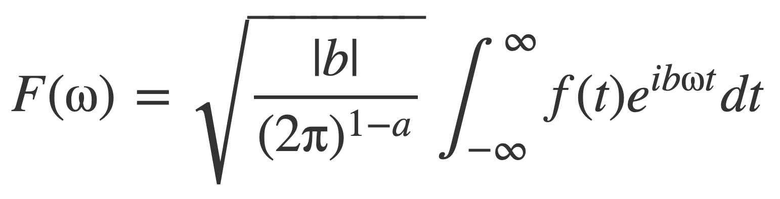
F(ω) is the frequency description of the function f(t), given by the Fourier transform of f(t), an improper integral:
![]()
The notation 𝓕[f(t)], or 𝓕, is used when referring to the Fourier transform as an operation, rather than the result F(ω) of the operation. Similarly the notation 𝓕 -1[F(ω)], or 𝓕 -1, is used when the inverse Fourier transform is considered an operation, rather than the result f(t):
F(ω) = 𝓕[f(t)](ω)
f(t) = 𝓕 -1[F(ω)](t)
The Fourier transform and inverse can also be expressed in terms of the oscillatory frequency components e-i2πft with the substitution ω = 2πf. A table for viewing some Fourier transforms, for both angular frequency ω and oscillatory frequency f, is at Fourier transform Table, some of which involve the Delta Function δ.
General Form of Fourier transform
The form of the Fourier transform 𝓕 has several variations but all lead to the same result as an inverse operation 𝓕 -1 that expresses a function as an integral of frequency components weighted by the values of its Fourier transform F(ω).
In Fourier transform at MathWorld it’s noted the general form of the Fourier transform can be expressed using a pair of numbers (a,b):
With inverse operation:
Choice of the Fourier transform
For consistency with the WolframAlpha examples used in this discussion the following form of the Fourier transform for a function f(t) is chosen, corresponding to (a,b) = (0,1):
![]()
The inverse operation is:
![]()
The notation f(t) ⇔ F(ω) is used for a Fourier transform pair.
Compare this form of the Fourier transform to that of the complex Fourier series:
![]()
Analogous to the DC component for Fourier series, the DC component corresponds to the zero frequency value of F(ω), or F(0):
![]()
A calculation of the Fourier transform as an extension of the complex Fourier series is presented in Lecture 8: Fourier transforms.
Fourier transform Existence Conditions
For constant and periodic functions the integral for the Fourier transform does not exist in the usual sense. The Delta Function is defined to extend its applicability to these functions.
In Fourier transform at MathWorld it is noted that the Fourier transform of f and its inverse exist under these conditions:
fis absolutely integrable: integral of the absolute value offon [-∞, ∞] is finite.fhas a finite number of discontinuities.fis of bounded variation.
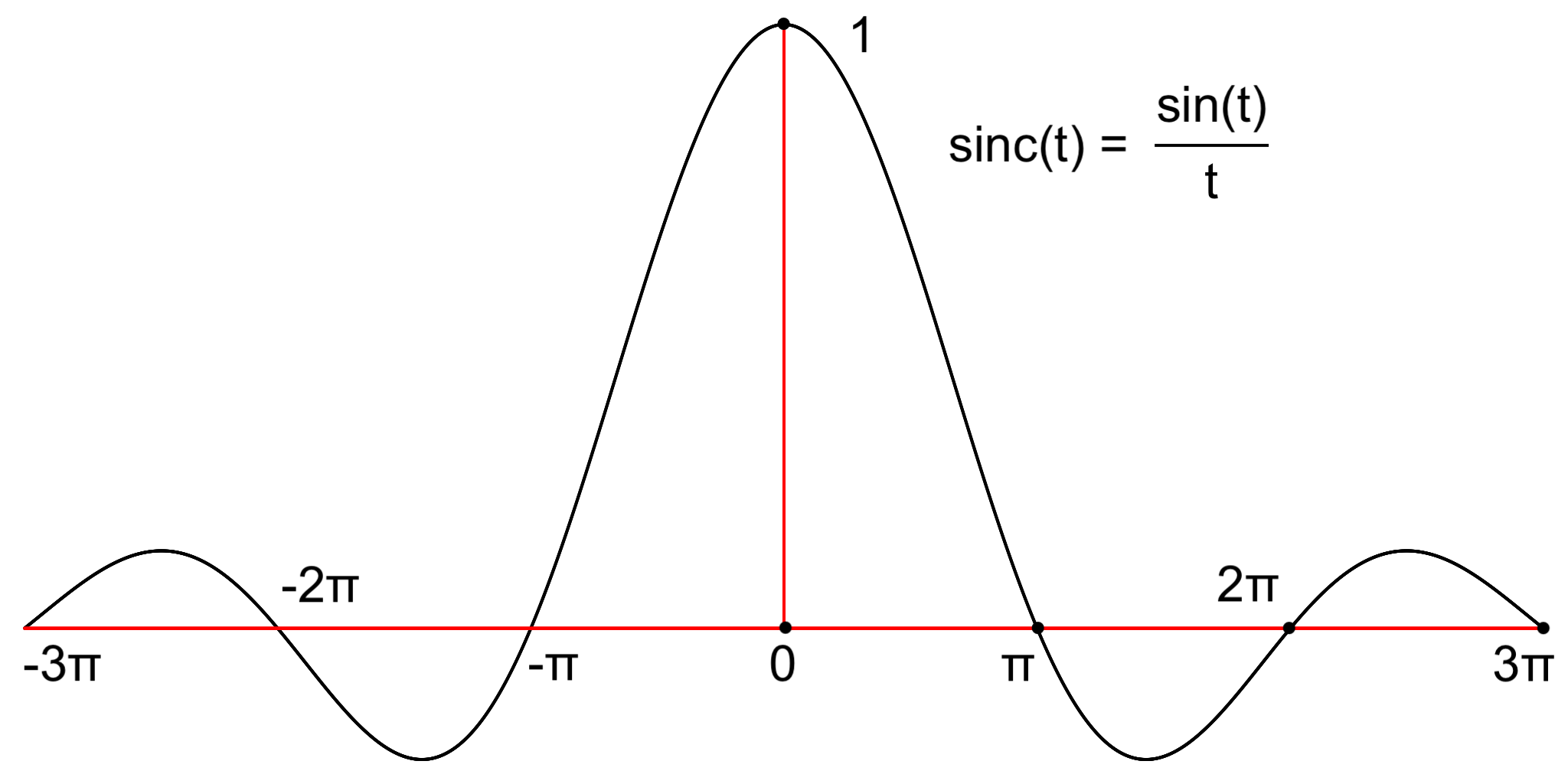
These conditions are not necessary. An example is the sinc function sinc, which plays an role in the derivation of the reconstruction formula for the Nyquist-Shannon sampling theorem. The sinc function is integrable but not absolutely integrable, yet the sinc function’s Fourier transform and inverse exist; see the calculation in Fourier transform of Sinc of Addendum About Sinc.
The property bounded variation is more restrictive than bounded. Intuitively a function has bounded variation on an interval [a,b] if doesn’t oscillate too much on [a,b]. If the arc length of a differentiable function is finite on [a,b] then it has bounded variation on [a,b].
Examples.
f(x) = sin(1/x), which oscillates an infinite number of times by the same amount near 0, is not of bounded variation on an interval containing 0:
The damped version of this function f(x) = x sin(1/x) also is not of bounded variation on an interval containing 0:

But the more damped version of this function f(x) = x^2 sin(1/x) is of bounded variation on an interval containing 0:

Notable Properties of the Fourier transform
Properties help find Fourier transforms using other known Fourier transforms. In the section Fourier transform of Sinc the Fourier transform of sinc function sinc is found from the Fourier transform of rectangle function rect using the duality and time scaling properties.
Additional properties are listed at Fourier transform properties and Fourier transform examples. A table of various Fourier transforms, for both angular frequency ω and oscillatory frequency f, is at Fourier transform Table.
Complex Valued
Notable Properties of the Fourier transform ↑
The Fourier transform F(ω) provides the weights of the components e-iωt for each real frequency ω as complex numbers. The modulus |c| of a complex number c = x + i y is given by:
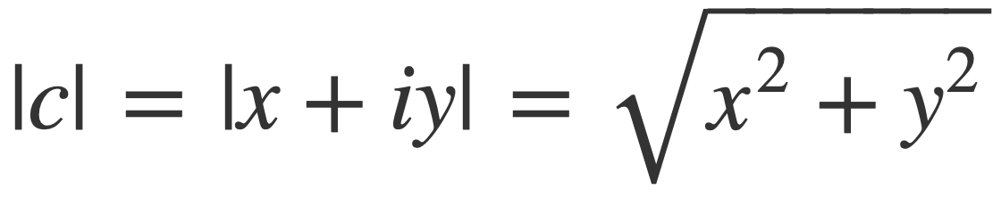
The modulus of F(ω) squared, |F(ω)|2, can be interpreted as energy density per frequency and a plot of |F(ω)|2 vs ω is used to visualize the frequency description F(ω).
Linearity
Notable Properties of the Fourier transform ↑
The Fourier transform is a linear operation:
𝓕[a f(t) + b g(t)] = a 𝓕[f(t)] + b 𝓕[g(t)]
Symmetry
Notable Properties of the Fourier transform ↑
For real valued time-domain signals f(t) the Fourier transform F(ω) is conjugate symmetric, meaning F(-ω) is the complex conjugate of F(ω). Therefore:
• |F(-ω)| = |F(ω)| (even)
• Re(F(-ω)) = Re(F(ω)) (even)
• Im(F(-ω)) = -Im(F(ω)) (odd)
Duality
Notable Properties of the Fourier transform ↑
If f(t) ⇔ F(ω), then F(t) ⇔ f(−ω)
To see this with the choice of the Fourier transform, start with the Fourier inversion formula:
![]()
Flip the symbols t and ω:
![]()
Negate ω:
![]()
But the right hand side is the just Fourier transform of F(t):
![]()
Time Scaling
Notable Properties of the Fourier transform ↑
If f(t) ⇔ F(ω), then f(kt) ⇔ F(ω/k)/|k|
This is the time scaling property, where expanding time compresses frequency, compare here with the Sinc and Rect Transform Pair:
![]()
Time scaling follows by an application of Change of Variables with g(t) = t/k, where when k < 0 the limits of integration of the improper integral flip from -∞,∞ to ∞,-∞. In this case the limits of integration are restored back to -∞,∞ by negating the integral, and is why the absolute value of k appears in the final result:
![]()
Vanishes at Infinity
Notable Properties of the Fourier transform ↑
By the Riemann-Lebesgue lemma if the integral of the absolute value of f on [-∞, ∞] is finite (f is absolutely integrable) then its Fourier transform F(ω) is continuous, and F(ω) → 0 as ω → ∞.
Uncertainty Principle
Notable Properties of the Fourier transform ↑
The uncertainty principle is that a function f(t) and its Fourier transform F(ζ) can not both be highly concentrated, a consequence of Heisenberg’s Inequality. The interpretation in physics is Heisenberg’s uncertainty principle.
The inequality is derived with the following alternate form of the Fourier transform F(ζ):
![]()
The statement involves the L2-norm of a complex valued function, a generalization of the norm of complex numbers, given by an integral over [-∞,∞]:
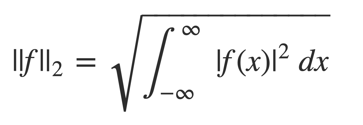
The norm of a complex number z = x + i y, denoted |z|, is given by:
Where:
And then:
Heisenberg’s Inequality, stated with proof in The Uncertainty Principle: A Mathematical Survey:
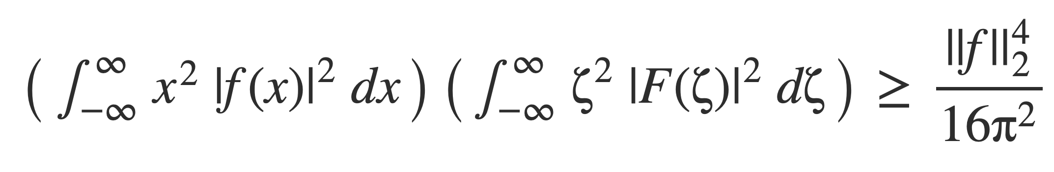
When the function f(t) has been normalized, so its norm ||f|| is equal to 1, then the right hand side simplifies:
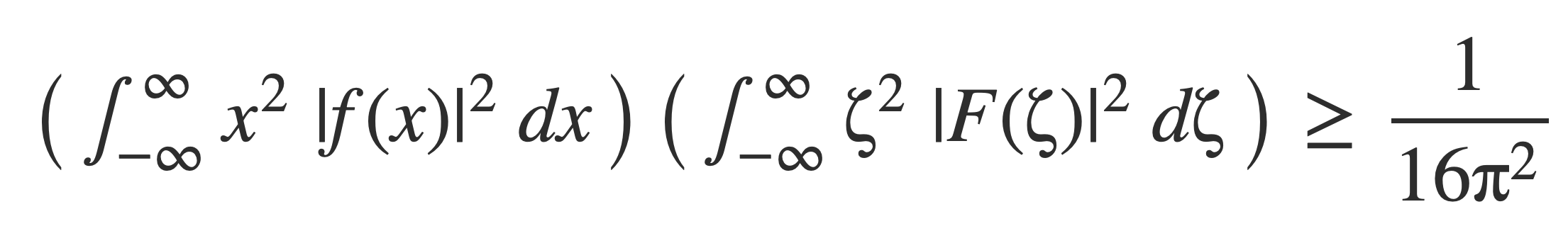
The integrals in the products on the left hand side are called variance of f and F, a measure how wide the functions are spread out from their average value. Since the product must remain bounded as it is, a decrease in the value of one may require an increase in value of the other.
Band-Limited Signals
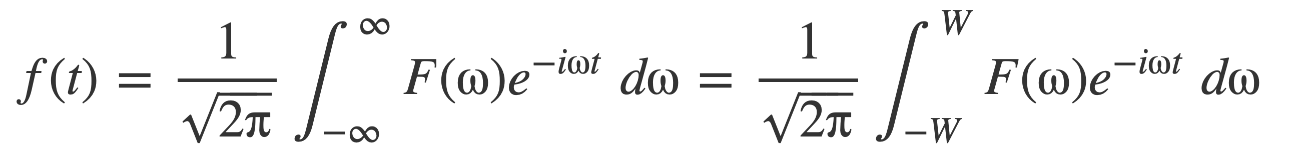
A function f(t) is band-limited if its Fourier transform F(ω) is zero outside a finite interval [-W, W], and time-limited when the function itself is zero outside a finite interval. When a function f(t) is band-limited to [-W, W] then it has no frequency components greater than W, and the inverse Fourier transform to recover f(t) is a finite rather than improper integral:
![]()
The sinc function is an example of a band-limited signal since its Fourier transform is the rectangle function rect, see Sinc and Rect Transform Pair. This Fourier transform pair illustrates the general property that band-limited signals are not time-limited.
In the case of a sinusoidal function like sine or cosine, which do not have a Fourier transform in the usual sense, the signal is band-limited to its single oscillatory frequency. The Fourier transform is extended to sinusoidal functions in Delta Function.
Sinc and Rect Transform Pair
In the section Fourier transform of Sinc the Fourier transforms of sinc function sinc and rectangle function rect are computed. The Fourier transform of rect is computed first and then the transform of sinc is computed using the duality and time scaling properties of Fourier transform.
The Fourier transform of the rect function is:
![]()
The Fourier transform of the sinc function is:
![]()
sinc is an example of an ideal band-limited signal, because its Fourier transform is the rect(t) function (also denoted by ∏), that is zero outside a finite interval:
Like all band-limited signals sinc(t) is of infinite duration:
Energy Spectral Density
Plancherel’s Theorem expresses the energy of a signal in terms of its Fourier transform F(ω). Specifically it equates the integral in the time domain ∫|f(t)|2dt for the total energy of a signal f(t) to the integral in the frequency domain ∫|F(ω)|2dω with its Fourier transform F(ω). This motivates the definition of the energy spectral density as |F(ω)|2.
In Compute Energy Spectral Density the Fourier transform of a decaying pulse vibration is computed and plotted for different rates of decay.
Power, Work and Energy
In a resistive electrical circuit if f(t) is a measurement of voltage over time then the squared values |f(t)|2 can be interpreted as power per sample because power P, voltage V, and resistance R are related by this equation:
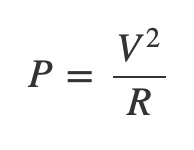
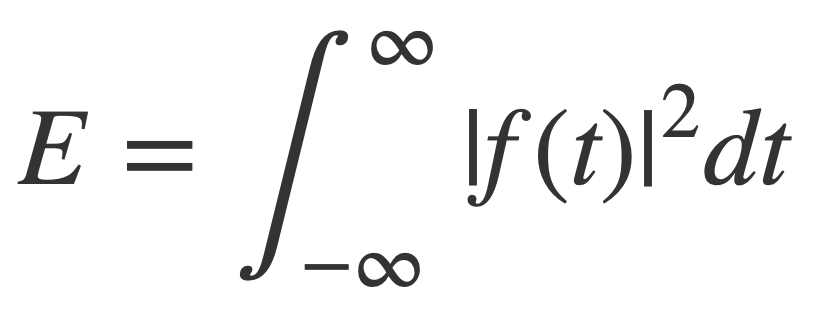
Since power P is the rate at which work W is done through the transfer of energy, so P = dW/dt or W = ∫ P(t) dt, the energy E of a function f(t) is defined as the integral of the its squared modulus over all time:
Plancherel’s Theorem
Plancherel’s Theorem is that the energy of a signal f(t) is preserved by its Fourier transform, through the following identity for a transform pair f(t) ⇔ F(ω):
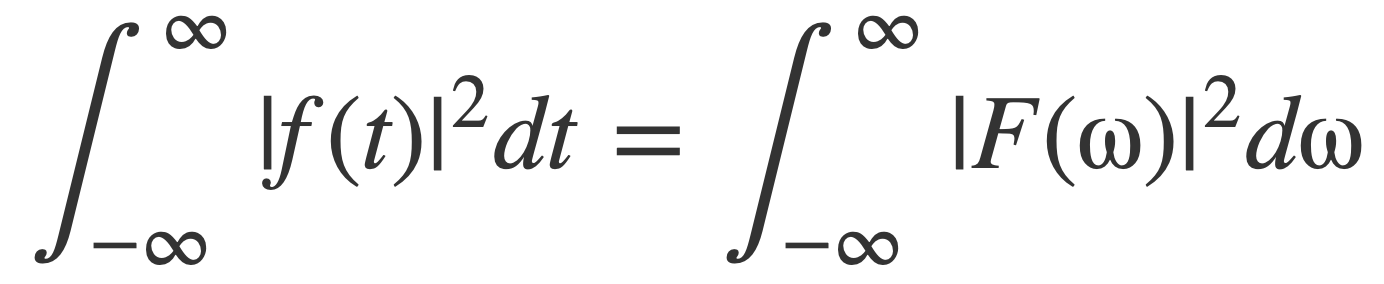
The interpretation is that the total energy of a signal, given by the left hand side as a sum of all power per sample, can also be computed using the values of its Fourier transform F(ω), and then |F(ω)|2 is interpreted as energy density per frequency.
When the concept of norm is extended from ordinary multidimensional vectors to functions, Plancherel’s Theorem expresses the norm preserving property of the Fourier transform.
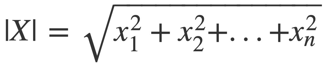
For a vector X of real values xi:
The norm |X| is given by:
The norm of a complex number z = x + i y, denoted |z|, is given by:
Where:
And then:
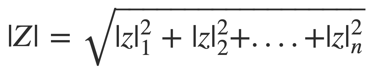
And for a vector Z of complex values zi:
The L2-norm of a complex valued function, a generalization of the norm of complex numbers, is given by an integral over [-∞,∞]:
Energy Spectral Density Definition
The energy E of a signal f(t),
is preserved under its Fourier transform by Plancherel’s Theorem,
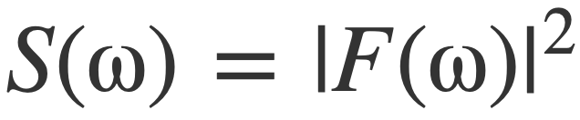
This equality that results in the energy interpretation of F(ω) as energy density per frequency motivates the definition of the energy spectral density S(ω) of a signal f(t) as the square of the modulus of its Fourier transform |F(ω)|:
Compute Energy Spectral Density
The Fourier transform of a decaying pulse vibration is computed and plotted for different rates of decay.
Define Model Signal
Compute Energy Spectral Density ↑
The model signal f(t) is a sine wave with angular frequency w, decaying exponentially with rate a, and zero for t < 0:
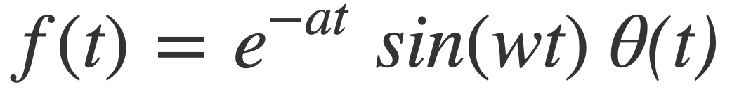
The Heaviside step function, or unit step function, denoted θ(t), limits the signal to t ≥ 0.
The expression for the model signal with values a = 2, w = (2 π 440) is:
Power[e,-2t] sin(2 π 440 t) θ(t)
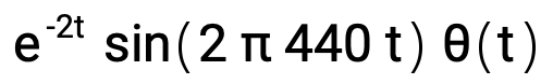
Plot the model signal on [ -0.5,0.5] by entering this expression:
plot Power[e,-2t] sin(2 π 440 t) θ(t) on -0.5,0.5
The decaying pulse vibration is plotted, zero for t < 0:
An audio file can be generated using the ToneWriter to play the sound of this function, where A0 = 440 Hz is the reference frequency commonly used to tune musical instruments:
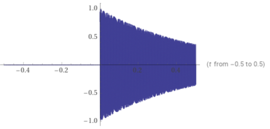
The value of t where the signal decays to essentially zero or 1/Int16.max = 1/32767 is calculated with the expression:
N[evaluate solve exp(-2t) = Divide[1,32767.0]]
The result is t ~ 5.19859, the chosen duration of the sample audio file. See GenerateTonePlayerSample for listing of the function GenerateTonePlayerSample() that generates the sample audio file, also included in the Xcode project.
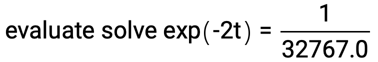
The duration t ~ 5.19859 is shown on the plot of e-2t here:
Compute the Fourier transform
Compute Energy Spectral Density ↑
The Fourier transform of the model signal is computed by entering this expression:
simplify FourierTransform Power[e,-at] sin(w t) θ(t)
![]()
The result when assuming a, w, ω positive is the Fourier transform F(ω) of the model signal f(t) is given by this expression:
Divide[w,(sqrt(2 π) (Power[w,2] + Power[(a - i ω),2]))]
![]()
Compute Modulus of the Fourier transform
Compute Energy Spectral Density ↑
Compute the modulus of the Fourier transform |F(ω)| of the model signal by entering this expression:
modulus(Divide[w,(sqrt(2 π) (Power[w,2] + Power[(a - i ω),2]))])
![]()
The modulus of the Fourier transform |F(ω)| is this expression:
Divide[sqrt(Power[w,2]),(sqrt(2 π) sqrt(4 Power[a,2] Power[ω,2] + Power[(Power[a,2] + Power[w,2] - Power[ω,2]),2]))]
![]()
Computation of Energy Spectral Density
Compute Energy Spectral Density ↑
The energy spectral density is the square of the modulus of the Fourier transform |F(ω)|2 computed by entering this expression:
Power[(modulus(Divide[w,(sqrt(2 π) (Power[w,2] + Power[(a - i ω),2]))])),2]
![]()
The result assuming a, w, ω positive is the Energy Spectral Density S(ω) of the model signal, given by this expression:
Divide[Power[w,2],2π(Power[(Power[a,2]+Power[w,2]-Power[ω,2]),2]+4Power[a,2]Power[ω,2])]
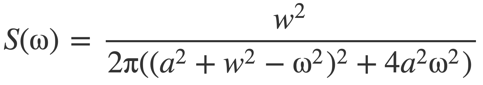
The energy spectral density S(ω) is a function of ordinary frequency f with the substitution ω = 2 π f.
Plot the Energy Spectral Density
Compute Energy Spectral Density ↑
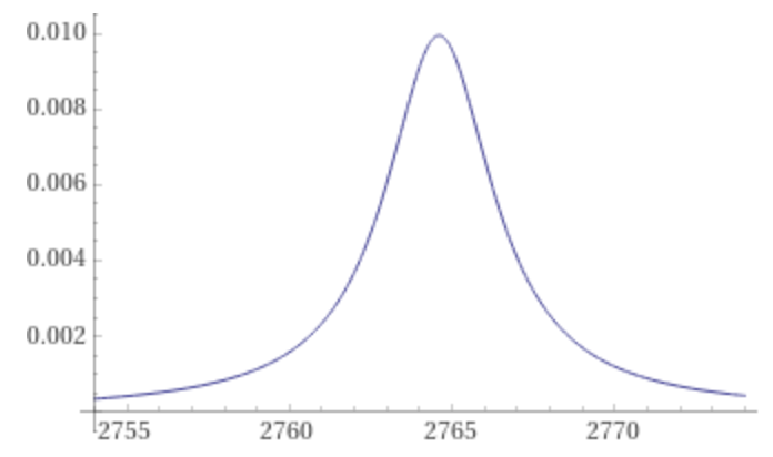
Plot the energy spectral density S(ω) by substituting the values a = 2, w = (2 π 440) with this expression:
plot Divide[Power[2 π 440,2],2π(Power[(Power[2,2]+Power[2 π 440,2]-Power[ω,2]),2]+4Power[2,2]Power[ω,2])] on 2764-10, 2764+10
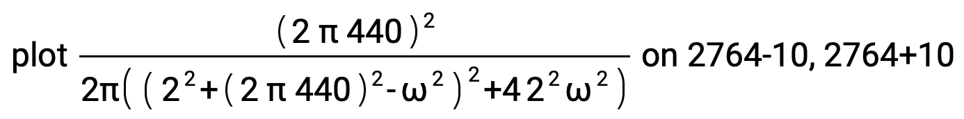
Plotted around the value w = (2 π 440) ~ 2764:
Also plot the energy spectral density S(f) by substituting ω = 2 π f into S(ω) with the same values a = 2, w = (2 π 440) with this expression::
plot Divide[Square[(2 π 4402)],2π(Power[(Power[2,2]+Power[2 π 440,2]-Power[2 π f,2]),2]+4Power[2,2]Power[2 π f,2])] on 440-1, 440+1
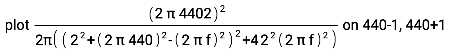
Plotted around the value f = 440:
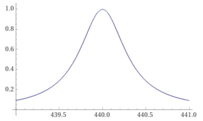
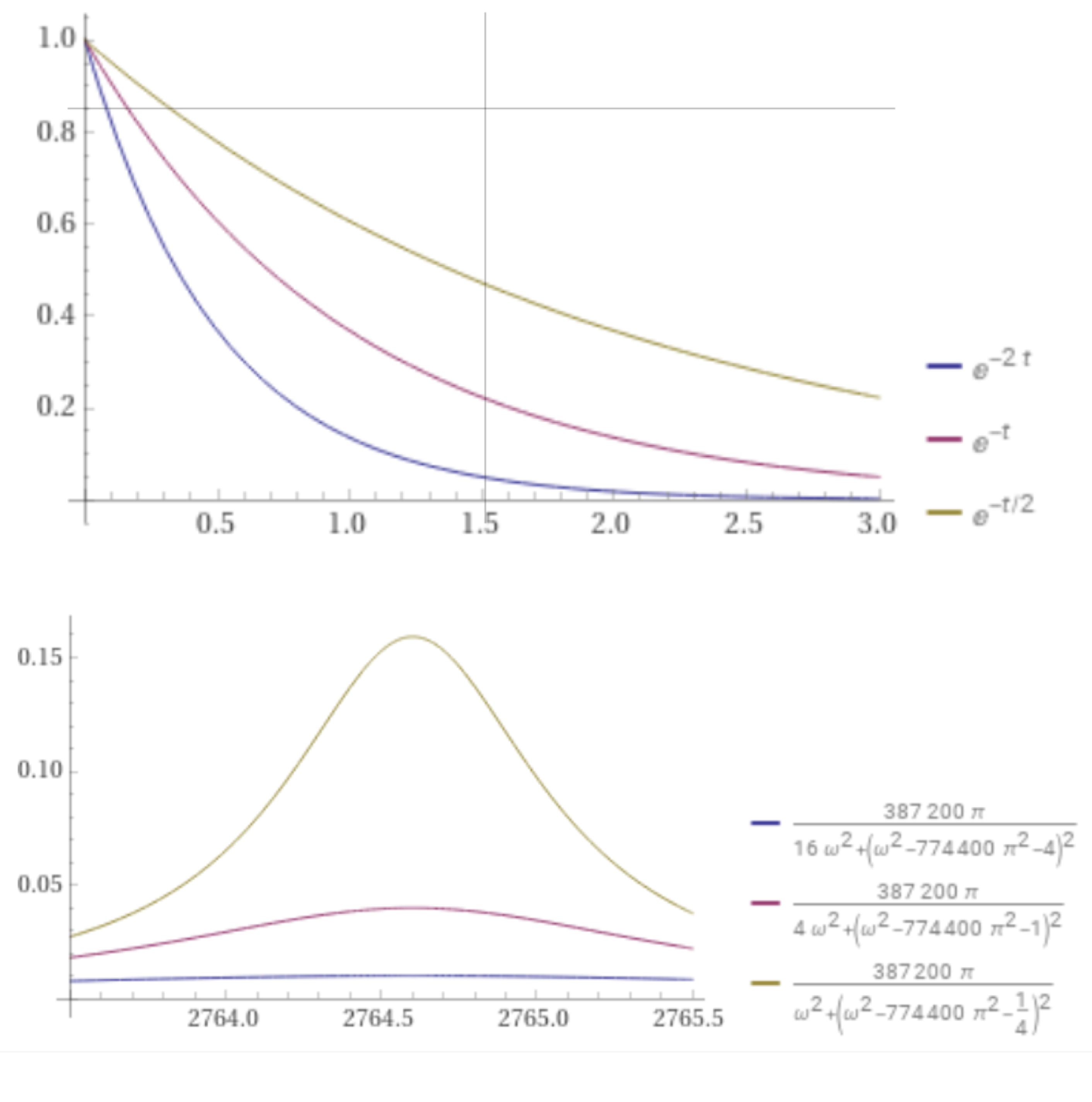
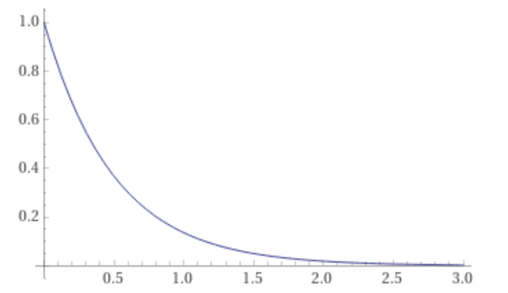
This is the energy spectral density of a sine wave that decays exponentially given by the model signal with a = 2, w = (2 π 440). The exponential decay is e-2t, plotted here with the expression:
plot Power[e,-2t] on 0,3
Verify Plancherel’s Theorem
Compute Energy Spectral Density ↑
Verify that the time domain and frequency domain calculations of energy for the model signal f(t) are the same.
The model signal f(t) is given by:
The energy spectral density S(ω) of the model signal f(t) is:
Plancherel’s Theorem is:
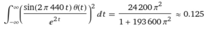
The integral of the model signal squared |f(t)|2 gives the total energy of the signal in the time domain, evaluated with this expression:
integrate Power[(Power[e,-2t] sin(2 π 440 t) θ(t)),2] on -∞, ∞

The result is 0.125:
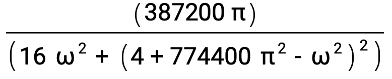
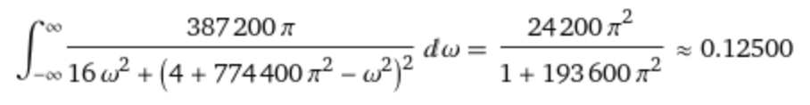
The integral of the energy spectral density S(ω) = |F(ω)|2 also gives the total energy of the signal in the frequency domain, evaluated with this expression:
integrate Divide[(387200 π),(16 Power[ω,2] + Power[(4 + 774400 Power[π,2] - Power[ω,2]),2])] on -∞, ∞

The result is also 0.125:
Compare Energy Spectral Densities
Compute Energy Spectral Density ↑
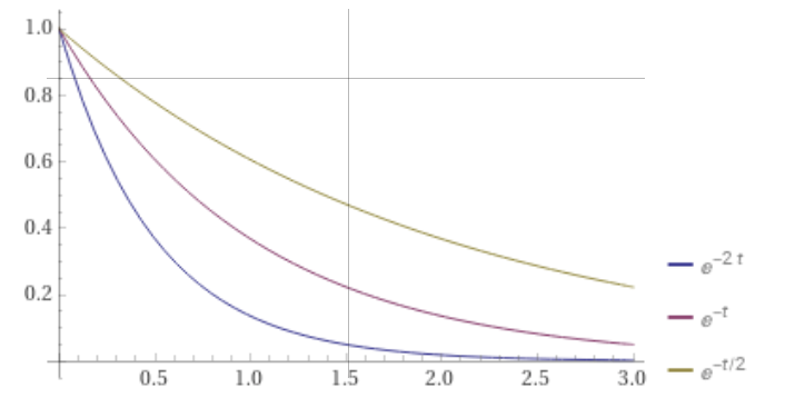
Create comparative plots as the rate of decay decreases, with a = 2, 1, and 0.5, by entering this expression:
plot Power[e,-2t] with Power[e,-t] with Power[e,-Divide[t,2]] on 0,3
The energy spectral density of given by:
Create comparative plots of the corresponding energy spectral density as the rate of decay decreases, a = 2, 1, and 0.5, and w = (2 π 440), entering this expression:
plot Divide[(387200 π),(16 Power[ω,2] + Power[(4 + 774400 Power[π,2] - Power[ω,2]),2])] with Divide[(387200 π),(4 Power[ω,2] + Power[(1 + 774400 Power[π,2] - Power[ω,2]),2])] with Divide[(387200 π),(Power[ω,2] + Power[(Divide[1,4] + 774400 Power[π,2] - Power[ω,2]),2])] on 2764.5 - 1, 2764.5+ 1
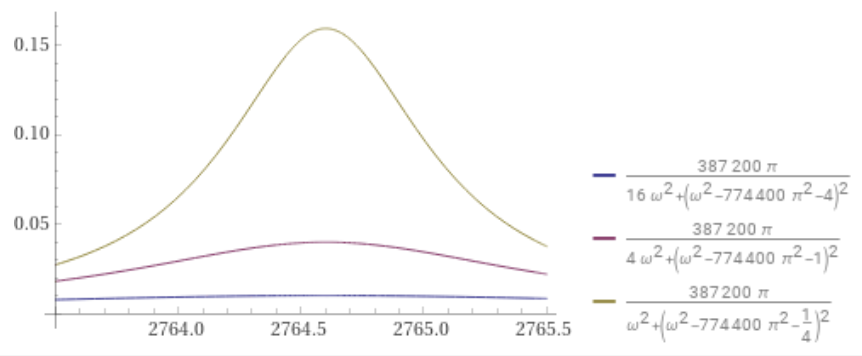
Blue curve → a = 2
Purple curve → a = 1
Gold curve → a = 1/2
The energy spectral density plots reveal more concentration near the angular frequency w = (2 π 440) = 2764 of the sinusoid sin(2 π 440 t) as the decay rate decreases from 2 to 1 to 1/2.
Delta Function
The Fourier transform of idealized constant and periodic functions f(t) do not exist in the usual sense because the transform integral for F(ω), an improper integral, does not converge. An extension of the Fourier transform to non-integrable functions is possible with the Dirac Delta Function δ.
Fourier transform of 1 and Dirac Delta Function δ
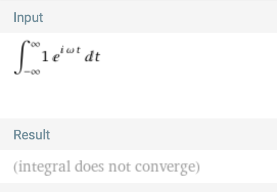
A function with a non-convergent Fourier transform is f(t) = 1:
integrate (1 Power[e,i ω t]) on -∞,∞

The response is integral does not converge:
However this expression is asking the same but differently:
FourierTransform 1
The response indicates the same integral is evaluated but returns a result with the δ function:
![]()
Fundamental Property of δ
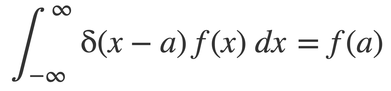
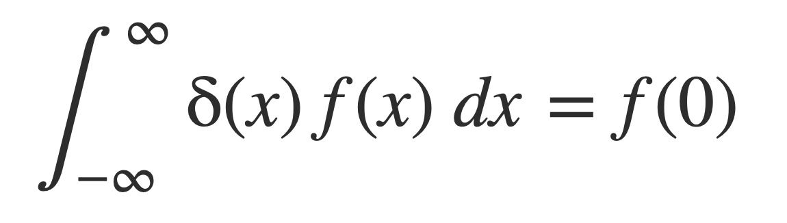
The Fundamental Property of δ, or sifting property, is that when a function f(x) is integrated alongside δ(x-a), then for any a the value of the integral is f(a):
In particular when a = 0:
Compute the inverse Fourier transform of δ, by entering this expression:
InverseFourierTransform Sqrt[2π]δ(ω)
![]()
This follows by applying the fundamental property of δ in the evaluation of the inverse Fourier transform integral, yielding the original function 1:
![]()
The following expression for the Fourier transform of the function 1,
![]()
is to be understood to mean that the inverse Fourier transform of the result returns the function 1, by applying the fundamental property of δ.
The Fundamental Property of δ can be viewed as a limit using Delta Sequences.
Delta Sequences
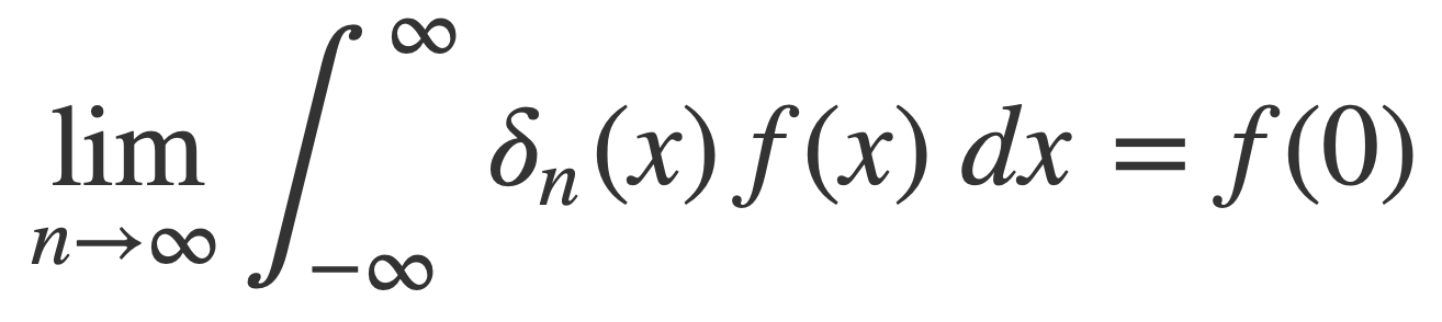
The δ function can be viewed as the limit of a sequence of ordinary functions δn(x) that converge through integration, rather than as a pointwise limit at each x. Pointwise convergence at x would mean that δn(x) → δ(x) as n → ∞. Instead a Delta Sequence is a series of functions δn(x) that converge in the sense of this limit:
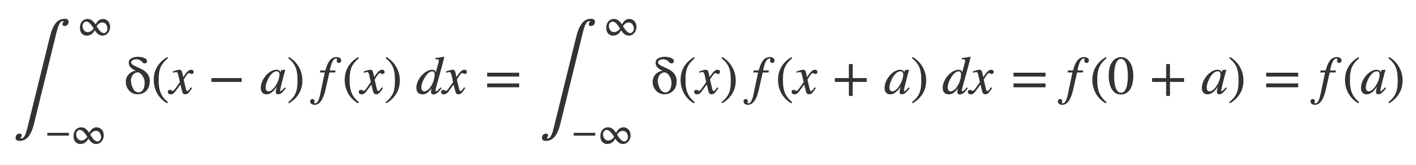
Then with a Change of Variables by setting g(x) = x+a, g’(x) = 1, the fundamental property should hold too:
The sequence δn are nascent delta functions, viewed as increasingly concentrated around zero, tending to infinity at zero, and converging to zero everywhere else (But the Sinc Nascent Delta Functions defined next, using the sinc function sinc, do not converge to zero for all non-zero values.)
Sinc Nascent Delta Functions
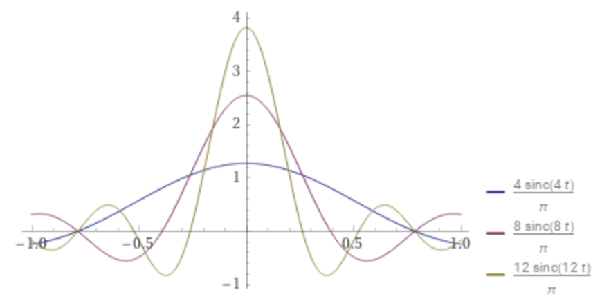
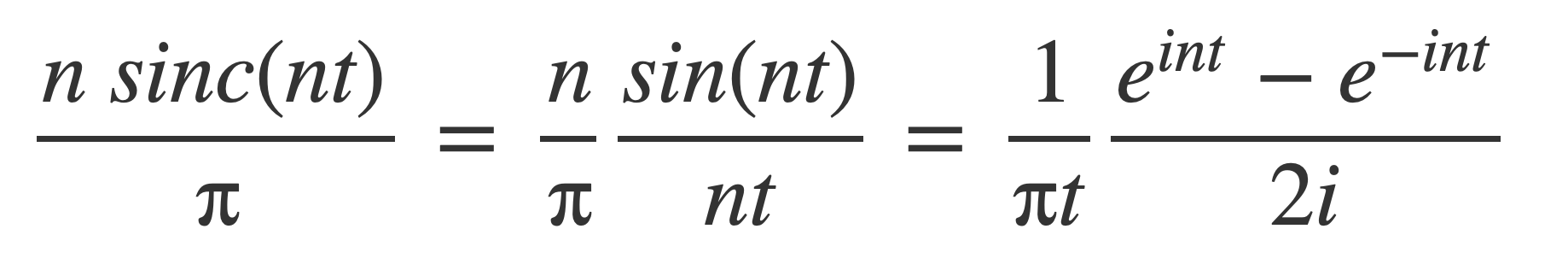
The sinc nascent delta functions δn are defined using the sinc function:
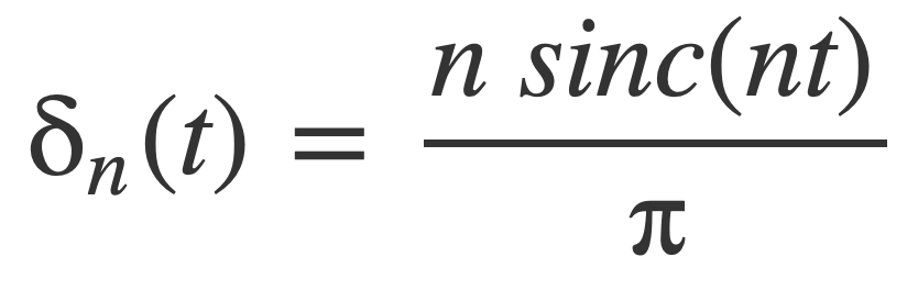
Plot some values of n, by entering this expression:
plot Divide[4,π] sinc(4t) with Divide[8,π] sinc(8t) with Divide[12,π] sinc(12t) on -1,1
For functions f that have a Fourier transform with an inverse, the δn are shown to have the nascent delta function convergence property:
The Fourier transform and its inverse are defined by these integrals:
![]()
Using Euler’s Formula:
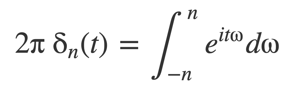
And then by the Fundamental Theorem of Calculus δn can be written as an integral:
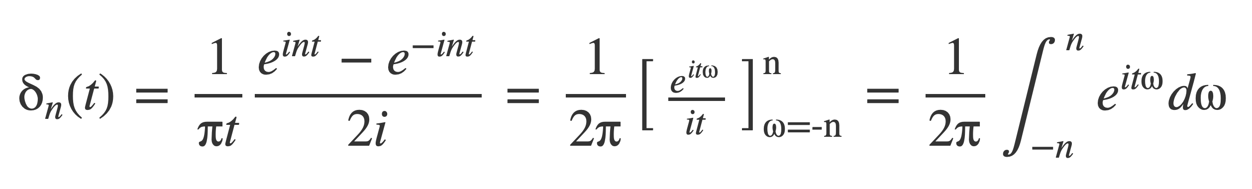
Suppose f(t) is a function that has a Fourier transform with an inverse, and substitute the previous expression for δn into the nth delta sequence integral:
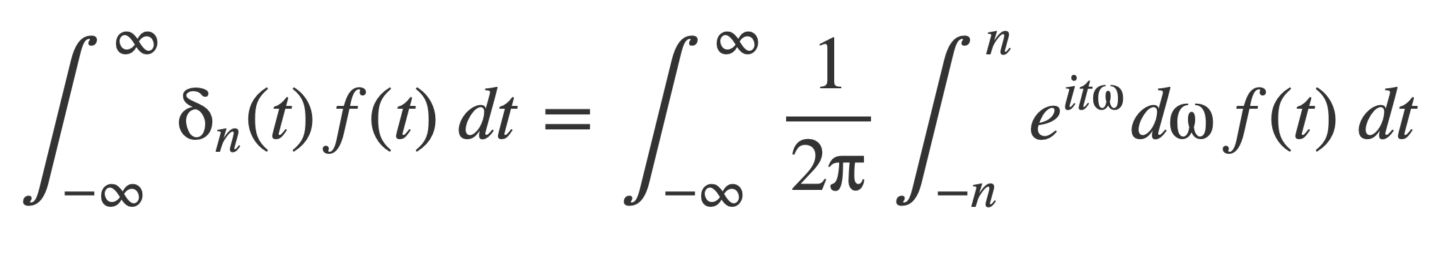
Change the order of integration, and factor 1/(2π) to rewrite the right hand side:
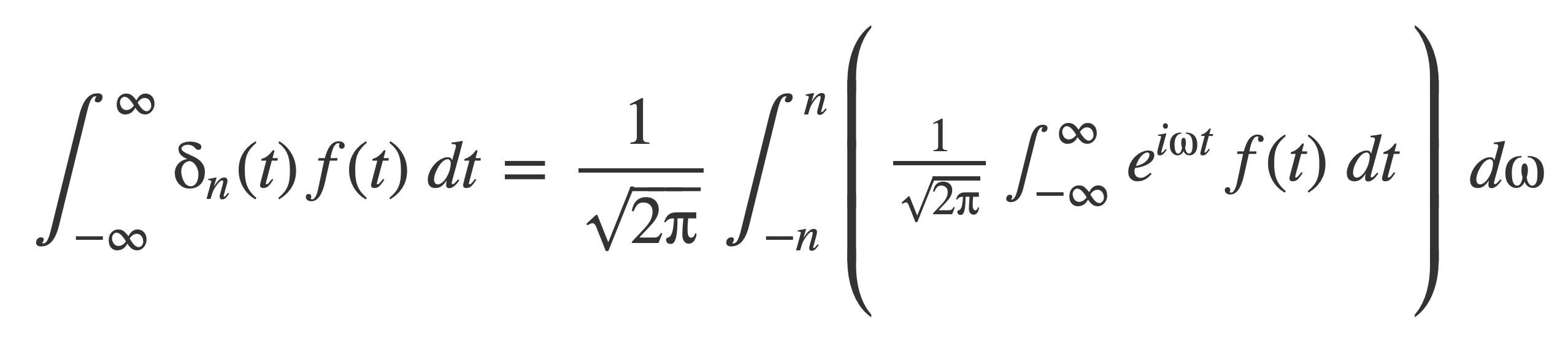
Since f(t) is a function that has a Fourier transform the inner bracket is the Fourier transform of f(t), 𝓕[f(t)] = F(ω). Substitute F(ω) and apply the limit n → ∞:
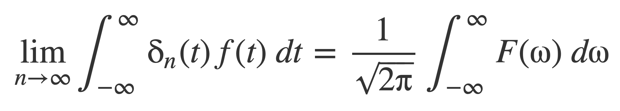
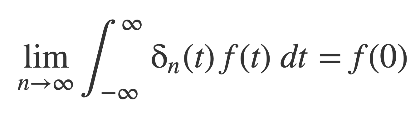
Since f(t) is a function that has an inverse Fourier transform, the right hand side is actually the inverse Fourier transform for f(t) evaluated at t=0, which is f(0):
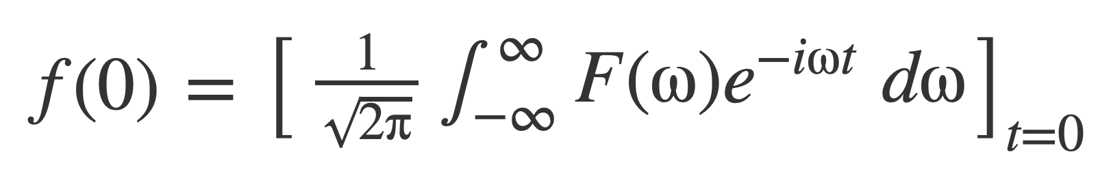
Therefore, if f(t) is a function that has a Fourier transform with an inverse, then δn converges to the δ function in the sifting property sense:
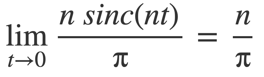
Also, δn tends to ∞ at zero. By L’Hôpital’s Rule, sinc(x) = sin(x)/x approaches 1 near 0:
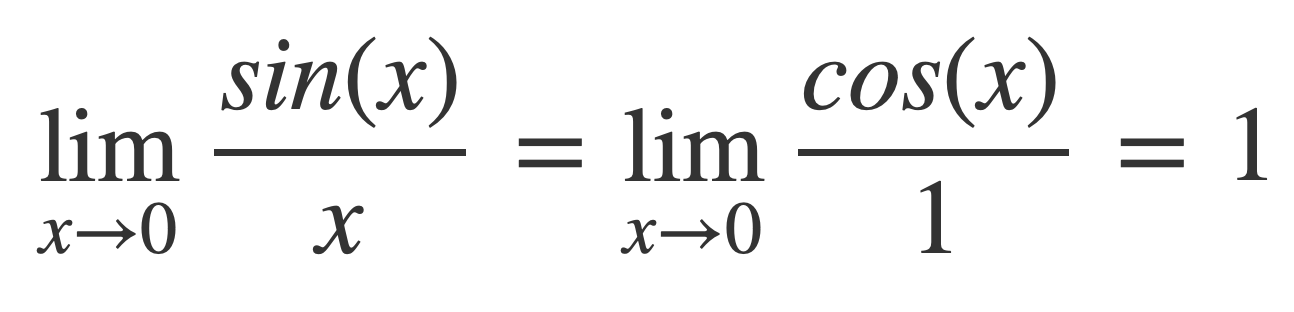
So then the following tends to ∞ at 0 as n does:
The sinc nascent delta functions provide an example of a sequence δn that does not converge to zero for all non-zero values of t. If t = π/2, for all odd n:
sin(n t) = sin(n π/2) = ±1
Then for all odd n:
n sinc(n π/2) = ±(2/π)
However n sinc(n t) tends to zero as t tends to infinity, given the bound:
|n sinc(n t)| = |n sin(n t)/(n t)| = |sin(n t)/t| < |1/t|.
Fourier transform of 1 Revisited
From Fourier transform of 1 and Dirac Delta Function δ, the Fourier transform of 1 is given by:
![]()
This claim is consistent with viewing δ as the limit of sinc nascent delta functions. Recall from Sinc Nascent Delta Functions that the sequence of sinc nascent delta functions δn can be expressed by an integral:
Or:
Use this to write the Fourier transform of 1 as the following limit:
![]()
Write this as:
![]()
Check this by substituting the limit of the sequence δn for δ in the integral for the inverse Fourier transform:
![]()
Or:
![]()
The integral on the right hand side,
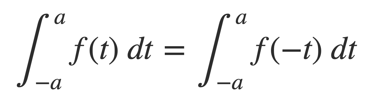
can be computed using the Fourier transform of the sinc function sinc, noting that for an integrable function f(t) and a:
In Fourier transform of Sinc it is shown that the Fourier transform of the sinc function sinc is:
![]()
Using the time scaling property and the symmetry of the rectangle function rect:
![]()
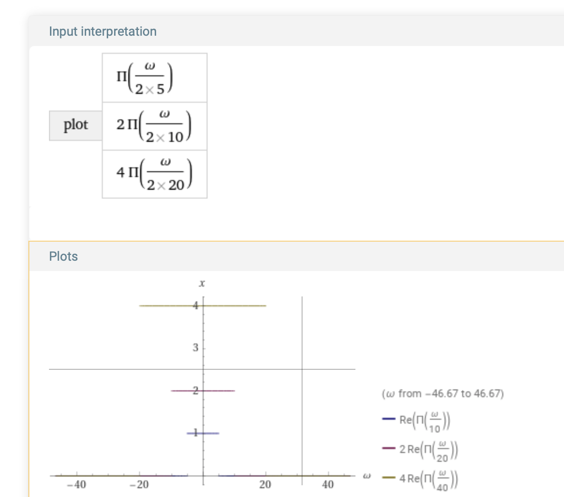
For n > 0 the function rect(ω/(2n)) is 1 on [-n,n] and 0 otherwise. Plot some scaled values to visualize, with the expression:
plot rect(Divide[ω,2 5]) with 2 rect(Divide[ω,2 10]) with 4 rect(Divide[ω,2 20])
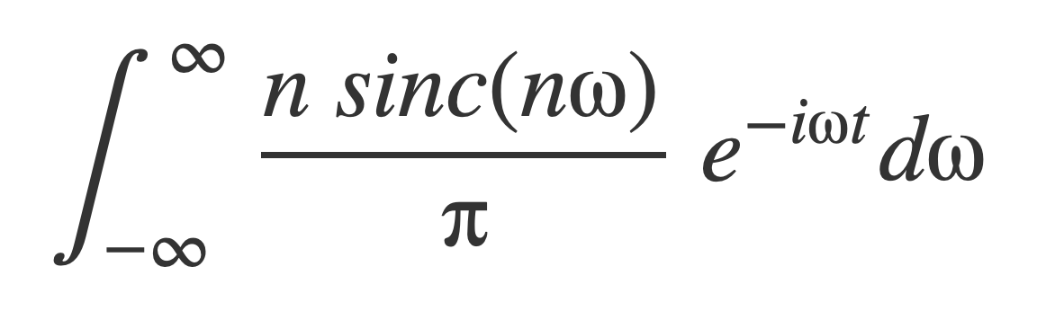
Substitute into the above expression for the inverse Fourier transform and evaluate the limit for n → ∞:
![]()
This result is consistent with the previous evaluation in Fourier transform of 1 and Dirac Delta Function δ using the sifting property of δ:
![]()
Or:
![]()
Fourier transform of Periodic Signals
Another function with a non-convergent Fourier transform is f(t) = sin(t), a periodic function with angular frequency ω = 1:
integrate (sin(t)Power[e,i ω t]) on -∞,∞

The response is integral does not converge:
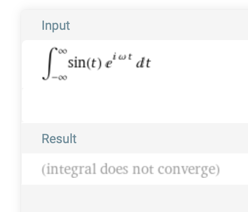
However this expression is asking the same but differently:
FourierTransform sin(t)
The response indicates the same integral is evaluated but returns a complex value involving two δ functions:
![]()
Fourier transform of Sine
Fourier transform of Periodic Signals ↑
The Fourier transform of sin(a t) can be evaluated using Euler’s Formula and 𝓕[1](ω).
First, using 𝓕[1](ω):
![]()
Then, using Euler’s Formula and linearity of 𝓕:
![]()
Simplifying yields 𝓕[sin(at)]:
![]()
Verify this by applying the inverse Fourier transform to the result, using the fundamental property of δ:
![]()
Fourier transform of Cosine
Fourier transform of Periodic Signals ↑
The Fourier transform of cosine will be computed using the Fourier transform of sine, the identity sin(t + π/2) = cos(t) and an identity for 𝓕[f(at+b)]:
FourierTransform f(at+b)
![]()
This follows by Change of Variables with g(t) = t - b/a:
![]()
And then:
![]()
Now use this result and the identity sin(t + π/2) = cos(t) to express 𝓕[cos(at)] in terms of 𝓕[sin(at)], that is already known:

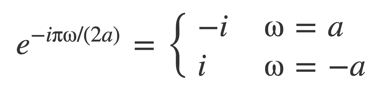
The exponential factor evaluates to these values for ω = a or ω = -a:
Substituting Fourier transform of sine, 𝓕[sin(at)]:
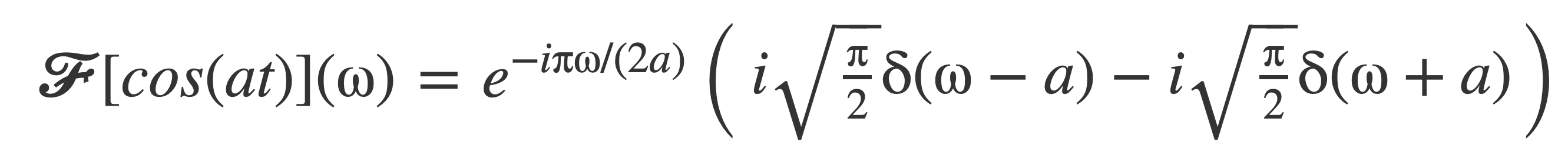
Distribute and replace the exponential with its values at ω = a or ω = -a by the sifting property of δ(ω - a) and δ(ω + a), respectively:
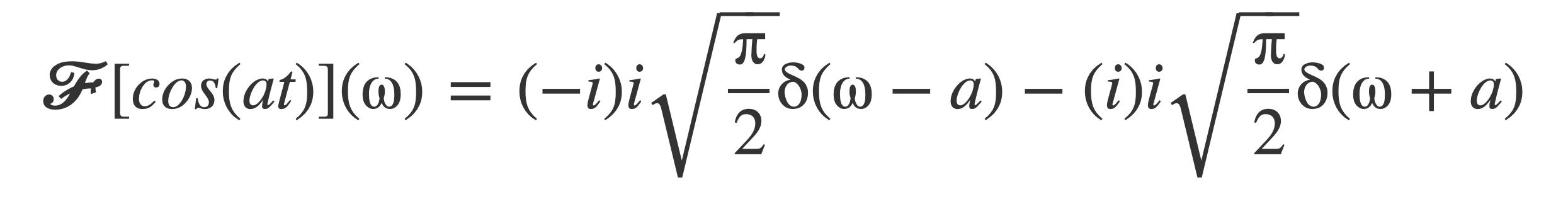
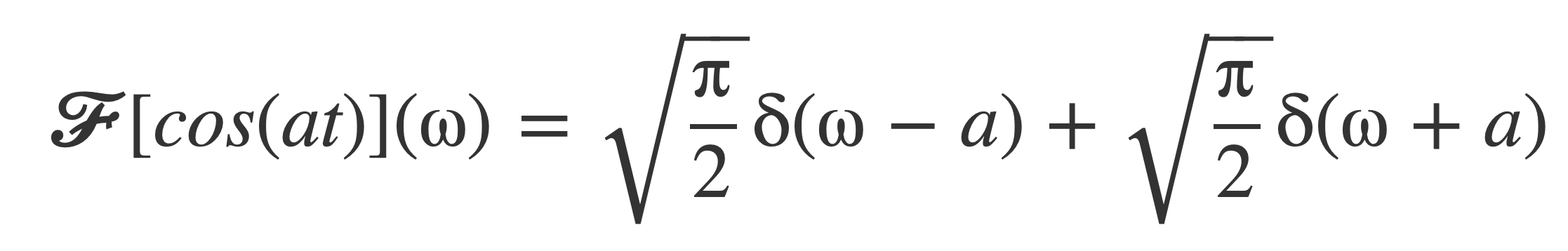
Substituting (-i)(i) = 1, (i)(i) = -1 yields 𝓕[cos(at)]:
Verify this by applying the inverse Fourier transform to the result, using the fundamental property of δ:
![]()
Fourier transform of Fourier series
Fourier transform of Periodic Signals ↑
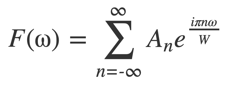
If the Fourier series of f(t) with fundamental frequency ω0 is:
Use linearity of 𝓕 to compute 𝓕[f(t)](ω):
![]()
Recall that:
![]()
Apply this to evaluate the Fourier transform of each complex exponential, yields 𝓕[f(t)]:
![]()
Nyquist-Shannon sampling theorem
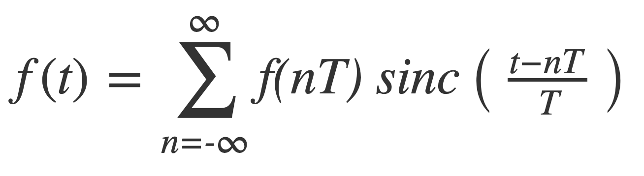
The classical form of the Nyquist-Shannon sampling theorem is a mathematical statement that says if a function with a Fourier transform is band-limited with maximum frequency B, then it can be exactly reconstructed from samples if the sample rate R is twice the maximum frequency B, or R = 2B. Given samples f(nT), n = …,-1,0,1,…, with uniform spacing T = 1/(2B) the reconstruction formula is:
with the normalized sinc defined as:
This formula is the Whittaker-Shannon interpolation formula which can be derived using the Fourier transform and its inverse. The frequency condition that F(ω) is zero outside [-B,B] enables the Fourier transform of the signal to be treated as a periodic function with a complex Fourier series, which is inverted term by term with the inverse Fourier transform to obtain the reconstruction formula.
In practice, the sample rate should be chosen strictly greater than twice the maximum frequency B, or R > 2B. Examples in Sampling Sinusoids show that sampling sinusoidal functions at a rate R such that R = 2B leads to significant aliasing.
In Sample Reconstruction the reconstruction formula is applied to three band limited signals: cos(t), the sinusoid sin(t), and the unnormalized sinc(t) = sin(t)/t. The implementation enables varying the number of terms in the partial sums for the infinite series, as well as B for varying the sample spacing T = 1/(2B), to draw plots that compare the reconstruction with the actual functions.
For an overview of the evolution of sampling theorems see Some Historic Remarks On Sampling Theorem.
Reconstruction Formula
Nyquist-Shannon sampling theorem ↑
The proof of the Nyquist-Shannon sampling theorem yields the Whittaker-Shannon interpolation formula:
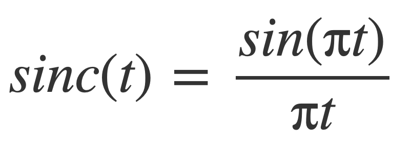
Where sinc is the normalized sinc function:
The derivation of the interpolation formula uses the same choice of the Fourier transform:
![]()
With inverse operation, given by the Fourier Inversion formula::
![]()
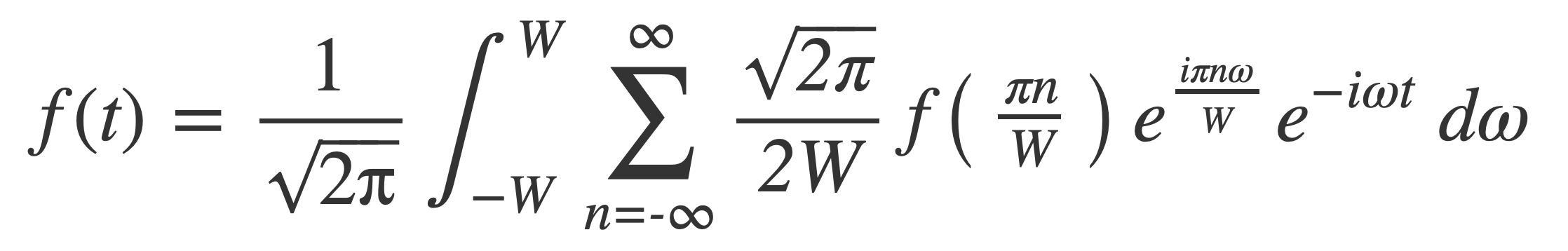
If the Fourier transform F(ω) of signal f(t) is zero outside [-W,W], W = 2 π B, then as a function with period 2W, F(ω) has a complex Fourier series, with W = L/2 or L = 2W:
Since F(ω) = 0 outside [-W,W] the coefficients An are given by:
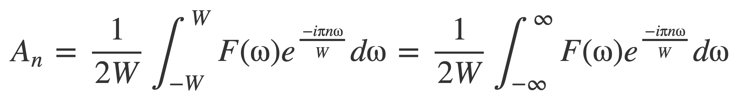
By the Fourier Inversion formula:
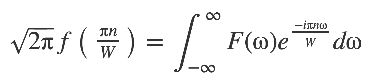
The coefficients An are then given by samples of f as:
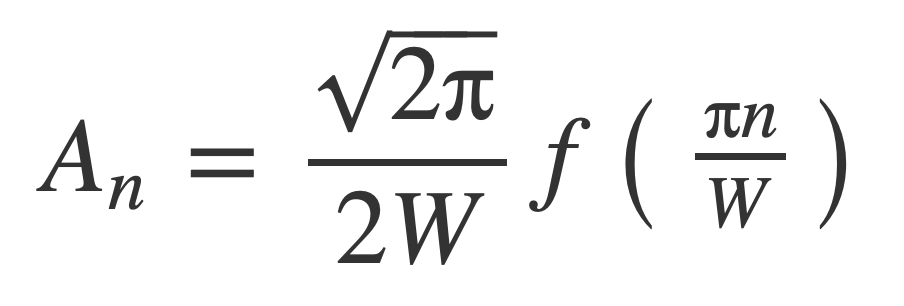
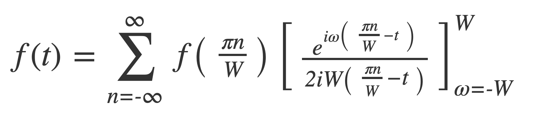
The Fourier transform F(ω) of f(t) has been expressed with samples of f(t) taken at multiples of π/W = 1/(2B) since W = 2 π B:
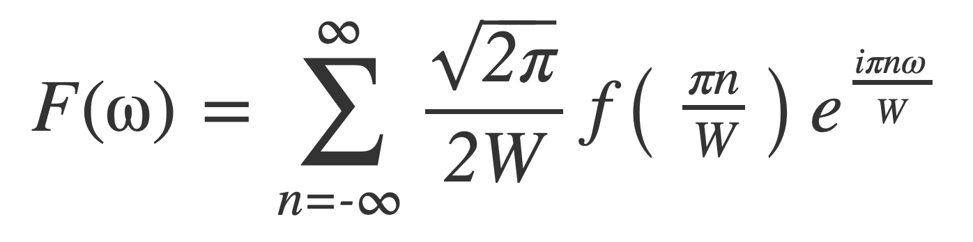
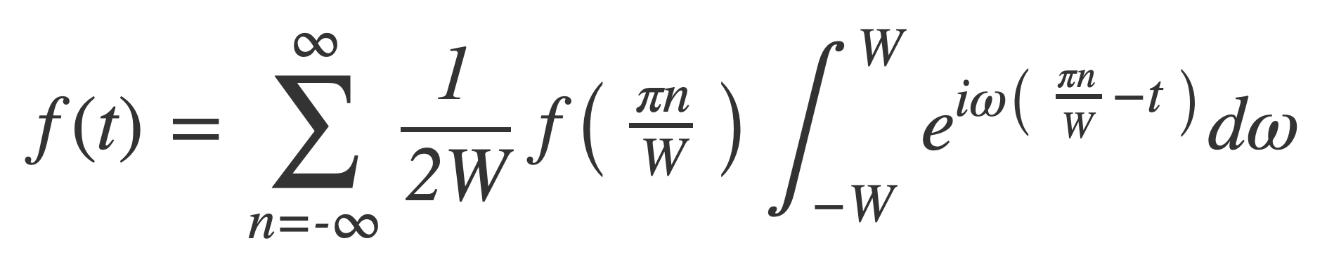
Apply the inverse Fourier transform 𝓕 -1 to both sides to recover f(t) from its samples. Using F(ω) = 0 outside [-W,W] :
Substitute the series expression for F(ω) with samples of f(t) at multiples of π/W:
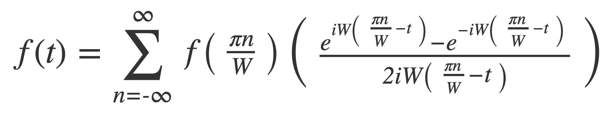
Switch the order of integration and summation, combine exponentials and simplify:
Evaluate the integral with the Fundamental Theorem of Calculus:
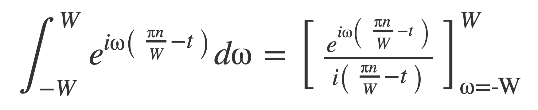
To obtain:
Expand the bracket:
Apply Euler’s Formula:
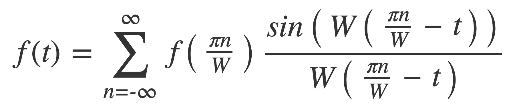
Convert from angular frequency to oscillatory with W = 2 π B:
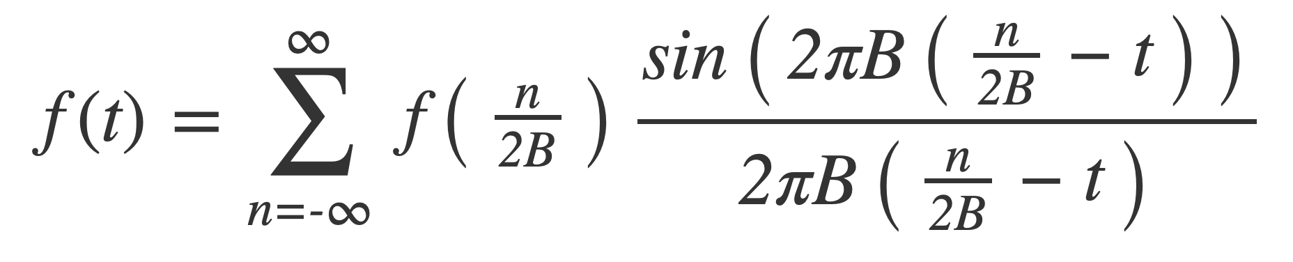
Substitute T = 1/2B for the spacing:
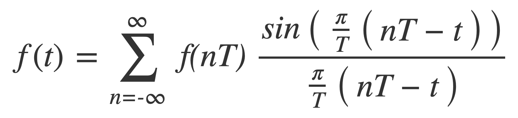
Finally substitute the symmetric sinc(t) = sin(πt)/πt to obtain the reconstruction formula:
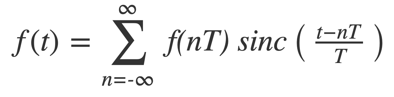
See Sample Reconstruction for an example applying the reconstruction formula to the band limited signal that is sinc(t) = sin(t)/t.
Nyquist frequency versus Nyquist rate
Nyquist-Shannon sampling theorem ↑
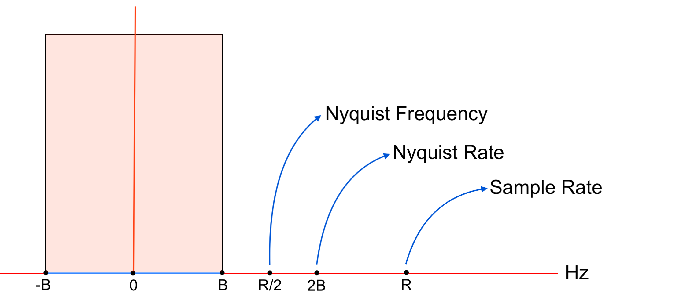
-
The Nyquist rate is the frequency that is twice the highest frequency
Bin the signal, or2B -
The Nyquist frequency is the frequency that is half the chosen sample rate
Rfor a signal, orR/2
Recall from the discussion in Tone Generation that the sampleRate is provided by AVAudioEngine at the time it is set up. The maximum tone frequency is then chosen as the Nyquist frequency corresponding to that sampleRate:
func highestFrequency() -> Double {
    return Double(sampleRate) / 2.0
}
Sampling Sinusoids
Nyquist-Shannon sampling theorem ↑
According to the Nyquist-Shannon sampling theorem the sample rate R should be strictly greater than twice the maximum frequency B, or R > 2B. Otherwise, if R = 2B, then aliasing can lead to a reconstructed signal that differs significantly from the original.
Example 1.
Sampling any sine wave at its corresponding Nyquist rate R = 2B will produces zeros, because sin(2 π B t) is zero for all n at t = n/(2B):
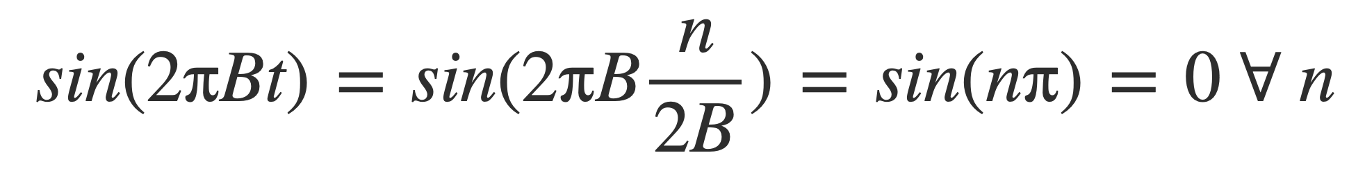
The signal sin(2 π t) with frequency 1 has maximum frequency B = 1. Let the sample rate R be twice the maximum so R = 2B = 2 * 1 = 2, so all samples are at multiples n of B/2 = 1/2:
n/2 = 0, 1/2, 1, 3/2, 2, ...
Sampling occurs at zero crossings of the signal where sin(2 π n /2) = sin(n π) = 0 for all integers n.
Also see the Sine Reconstruction Screenshots in the Sample Reconstruction section.
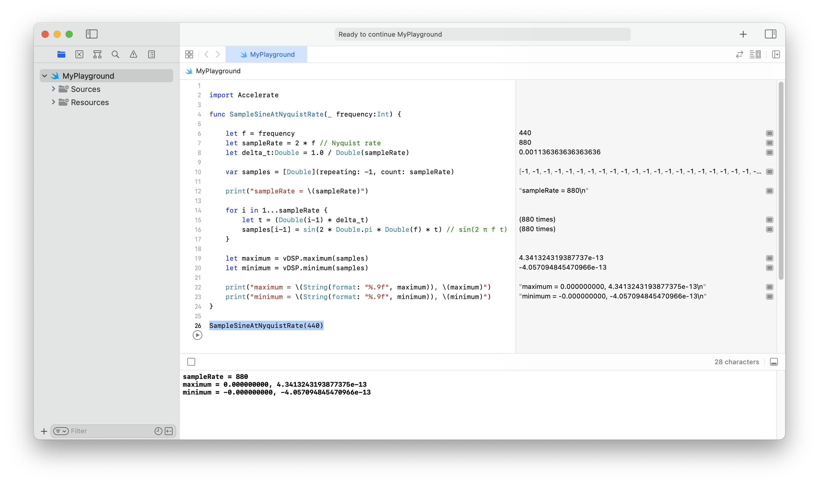
Code Experiment. The function SampleSineAtNyquistRate samples a sine wave at its Nyquist frequency. The samples are essentially all zeros, checked with the maximum and minimum functions of vDSP in the Accelerate framework:
import Accelerate

func SampleSineAtNyquistRate(_ frequency:Int) {

    let f = frequency
    let sampleRate = 2 * f // Nyquist rate
    let delta_t:Double = 1.0 / Double(sampleRate)

    var samples = [Double](repeating: -1, count: sampleRate)

    print("sampleRate = \(sampleRate)")

    for i in 1...sampleRate {
        let t = (Double(i-1) * delta_t)
        samples[i-1] = sin(2 * Double.pi * Double(f) * t) // sin(2 π f t)
    }

    let maximum = vDSP.maximum(samples)
    let minimum = vDSP.minimum(samples)

    print("maximum = \(String(format: "%.9f", maximum)), \(maximum)")
    print("minimum = \(String(format: "%.9f", minimum)), \(minimum)")
}
Running SampleSineAtNyquistRate(440) in an Xcode playground:
Example 2.
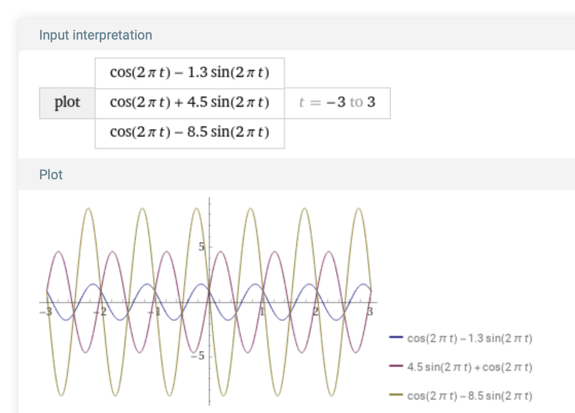
Signals of the form f(t, k) = cos(2 π B t) - k sin(2 π B t) build on the previous example. This collection of signals are aliases of each other when the sample rate is such that R = 2B: Since cos(nπ) = (-1)n and sin(nπ) = 0 for all n, then f(n/(2B), k) = (-1)n, for all n and all k.
For example, plotting these functions with B = 1, so 1/(2B) = 1/2, and k = 1.3, -4.5 and 8.5:
plot (cos(2 π t) - 1.3 sin(2 π t)) with (cos(2 π t) + 4.5 sin(2 π t)) with (cos(2 π t) - 8.5 sin(2 π t)) on -3,3
The identical samples occur at the intersections of the plots, which are all multiples of 1/2:
Sample Reconstruction
Nyquist-Shannon sampling theorem ↑
According to the Nyquist-Shannon sampling theorem the Whittaker-Shannon interpolation formula can be used to reconstruct a function from its samples when it has a band limited Fourier transform. A SwiftUI implementation of the experiment at Reconstructing a Sampled Signal Using Interpolation is used to reconstruct the three signals cos(t), sinc(t) = sin(t)/t, and sin(t) from samples taken at an adjustable rate to see the effect on the plots. The highest frequency, or bandwidth, of signals are determined from their Fourier transforms, and converted to oscillatory frequency (Hz) as the initial values for sample rate. As it turns out these three signals have the same bandwidth, ~ 0.16 Hz.
Determine Signal Bandwidths
Cosine Bandwidth For Reconstruction
The cosine, as a periodic function, requires delta functions to express its Fourier transform. See Fourier transform of Periodic Signals in the Delta Function section.
![]()
With ω = 1 = 2 π f as the highest frequency in the signal, f = 1/(2π), and cos(t) has bandwidth B = 1/(2π) ~ 0.16 Hz.
Sinc Bandwidth For Reconstruction
The (un-normalized) sinc function sinc(t) = sint(t)/t has a Fourier transform in the usual sense. See Fourier transform of Sinc in the Addendum About Sinc.
![]()
The Fourier transform of sinc is proportional to the rectangle function rect, which is non zero on [-1/2, 1/2]. With ω = 1 = 2 π f as the highest frequency in the signal, f = 1/(2π), and sinc(t) = sint(t)/t has bandwidth B = 1/(2π) ~ 0.16 Hz.
Sine Bandwidth For Reconstruction
The sine, as a periodic function, requires delta functions to express its Fourier transform. See Fourier transform of Periodic Signals in the Delta Function section.
![]()
With ω = 1 = 2 π f as the highest frequency in the signal, f = 1/(2π), and sin(t) has bandwidth B = 1/(2π) ~ 0.16 Hz.
However, as noted in Sampling Sinusoids:
The sample rate R must be strictly greater than twice the maximum frequency B, or R > 2B. If the sample rate R is chosen to be exactly 2B, the Nyquist rate, aliasing occurs and the reconstructed signal differs significantly from the original.
The Sine Reconstruction Screenshots illustrate the degeneration of the reconstruction when the sample rate R is chosen to be exactly 2B, namely 0.16 Hz.
Code Snippet For Reconstruction
Following is the code snippet that implements the reconstruction formula, where B is initialized to the actual bandwidth of the signal initially, which is ~0.16 Hz in both cases. The value B can be adjusted with a slider to effectively change the sample rate to test under-sampling and over-sampling the signal for reconstruction. The number of terms N in the partial summation of the infinite reconstruction formula is also adjustable with a slider.
    @Published var B = 0.16  // ~ 1.0/(2 * .pi)
    @Published var N = 10.0
    @Published var signalType = SignalType.sinc
...

    /*
     For both sinc(t) and cos(t) B = 1/(2 π) ~ 0.16

     • sinc(t) [unnormalized]
        For sinc(t) with FourierTransform is (sqrt(π/2) rect(ω/2)) ->
        rect(π f), solve π f = 1/2, f = 1/(2 π) ~ 0.16

     • cos(t)
        B =  2 π f = 1,  f = 1/(2 π) ~ 0.16
     */

    func sinc(_ t:Double) -> Double {
        if t == 0 {
            return 1
        }

        return sin(t) / (t)
    }

        // signal to sample
    func signal(_ t:Double) -> Double {
        switch signalType {
            case .cosine:
                return cos(t)
            case .sinc:
                return sinc(t)
            case .sine:
                return sin(t)
        }
    }

        // reconstruct signal
    func reconstruction(_ t:Double) -> Double {
        var sum:Double = 0

        let nbrTerms = Int(N)

        for i in -nbrTerms...nbrTerms {
            let n = Double(i)
            sum += signal(n/(2 * B)) * sinc( .pi * (2 * B * t - n))
        }

        return sum
    }
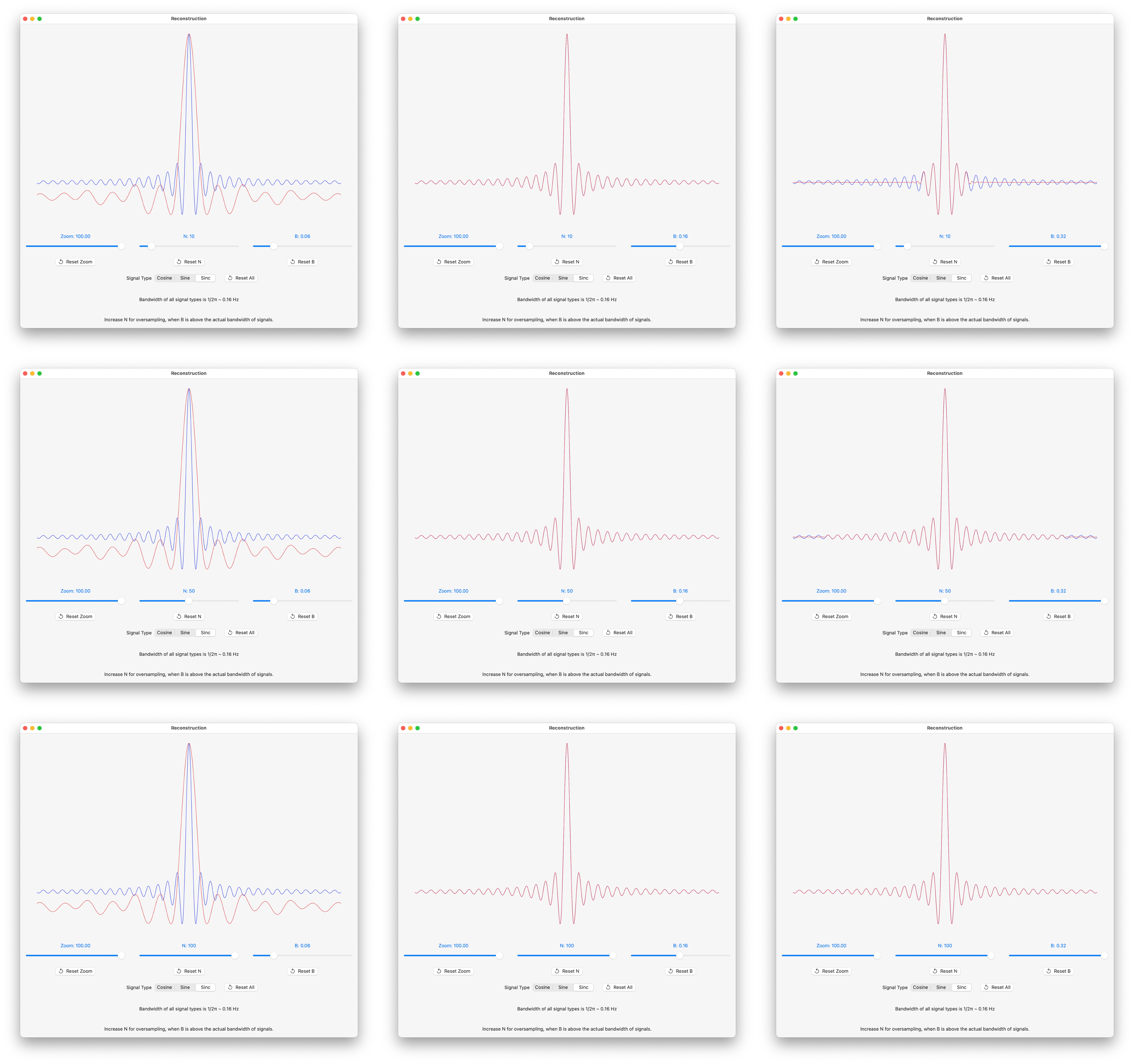
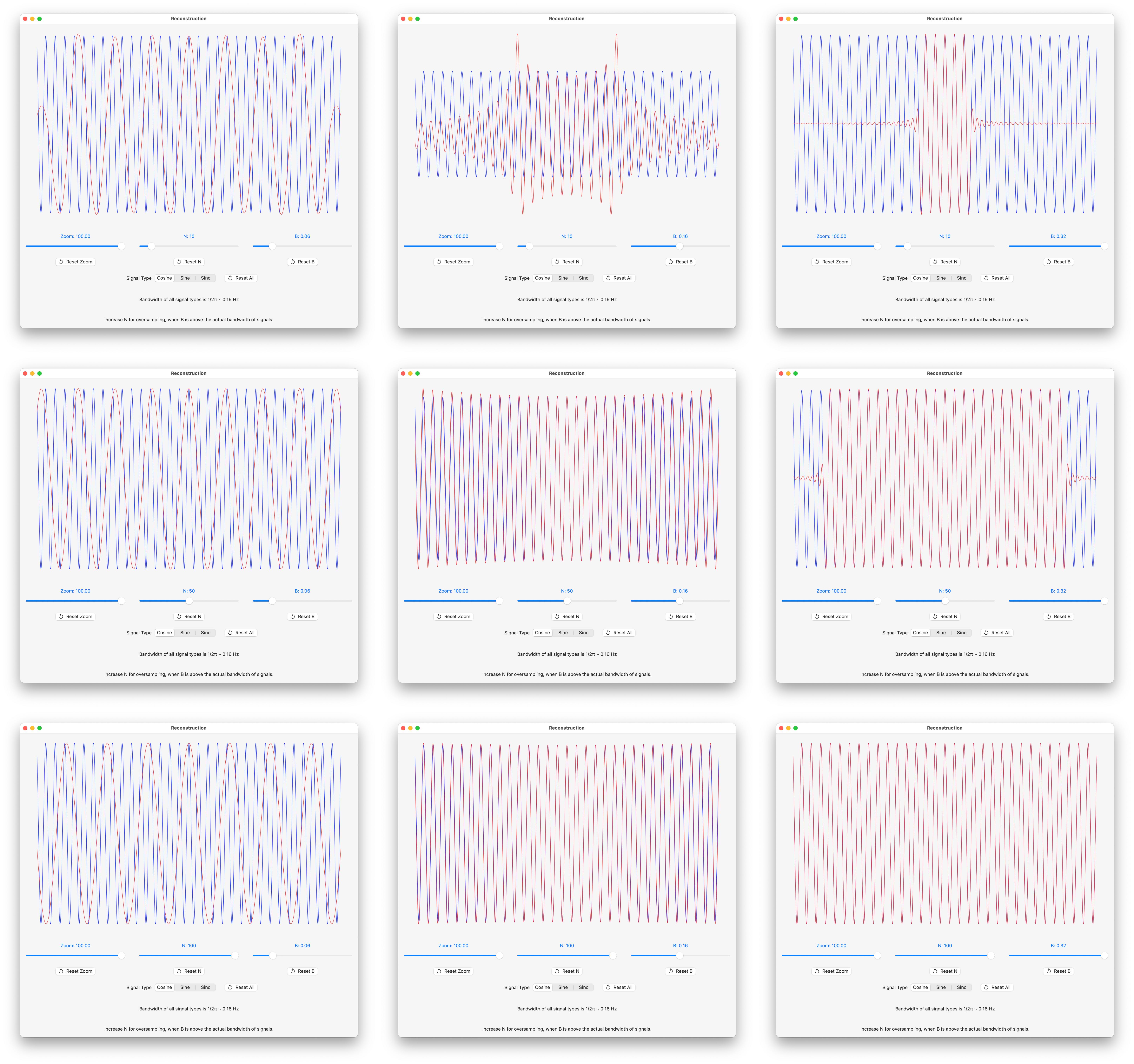
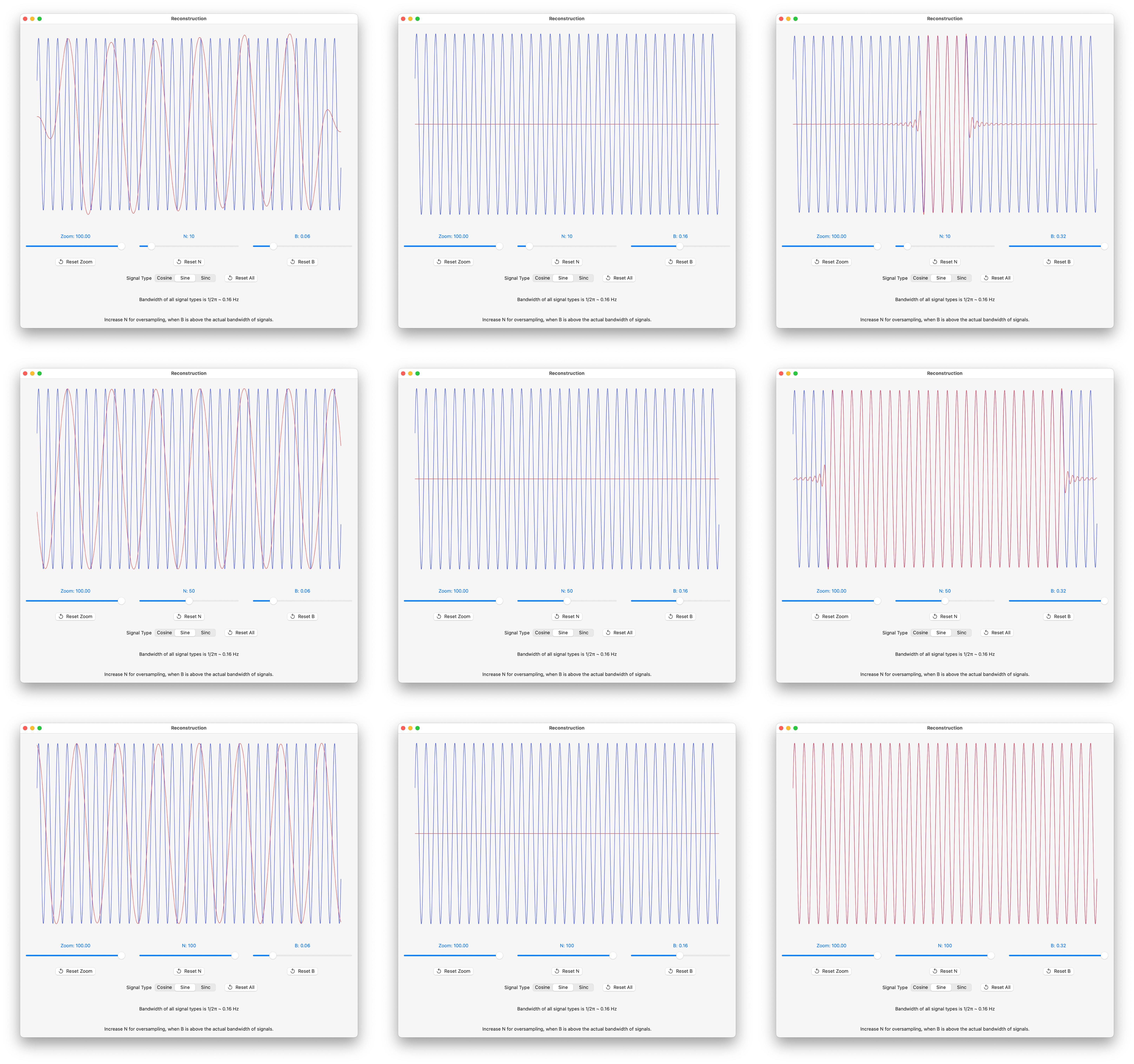
Signal Reconstruction Screenshots
Screenshots where:
• B, that determines sample spacing as T = 1/2B, varies left to right : 0.06, 0.16 and 0.32.
• N, number of partial sum terms, varies top to bottom: 10, 50 and 100.
The red curve is the plot of the reconstruction, the blue curve is the actual function.
Sinc Reconstruction Screenshots
Cosine Reconstruction Screenshots
Sine Reconstruction Screenshots
The reconstruction degenerates when the sample rate R is chosen to be exactly 2B, namely 0.16 Hz. It was noted in Sampling Sinusoids that all samples are zero in this case, and the reconstruction is a flat line in the center column screenshots.
Addendum About π
“I learned very early the difference between knowing the name of something and knowing something.” ― Richard P. Feynman
Archimedes’ calculation of pi in the 3rd century B.C. predates but shares concepts of calculus developed in the late 17th century, particularly the concept of limit. Using plane geometry and calculus, without trigonometry, it can be seen that for any circle the ratio C/d of length of its circumference C to diameter d is the same number named π.
Pythagorean theorem
The Pythagorean theorem is that for a right triangle with sides a, b and hypotenuse c,
a2 + b2 = c2

To see this construct the following diagram:
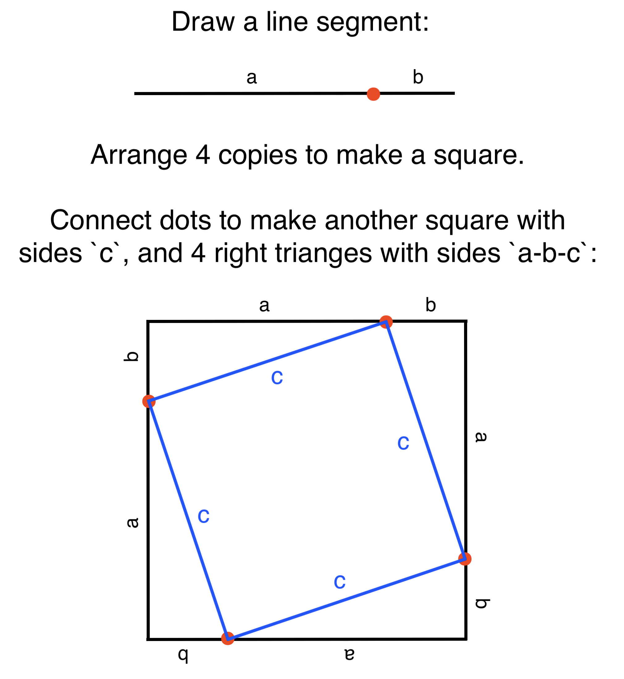
In the diagram the area of the outer square is (a+b)2, the area of the inner square is c2, and the area of each right triangle is ab/2. The area of the outer square is the sum of the areas of the inner square and all 4 right triangles:
(a+b)2 = c2 + 2ab
Or:
c2 = (a+b)2 - 2ab = b2 + 2ab + a2 - 2ab
The terms 2ab cancel out yielding:
c2 = a2 + b2
Definition of Arc Length
First motivate the definition of the length of the circumference C of a circle.
Given a differentiable function f(x) the length of the path of coordinates (x, f(x)) it traces as x varies over some interval [a,b] is approximated using a series of line segments. This is done by connecting the adjacent points formed by a grid of points spaced by Δ in the interval.
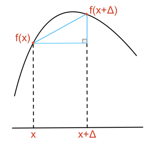
Using the Pythagorean theorem the total length in this approximation is the sum S over a partition of [a,b]:
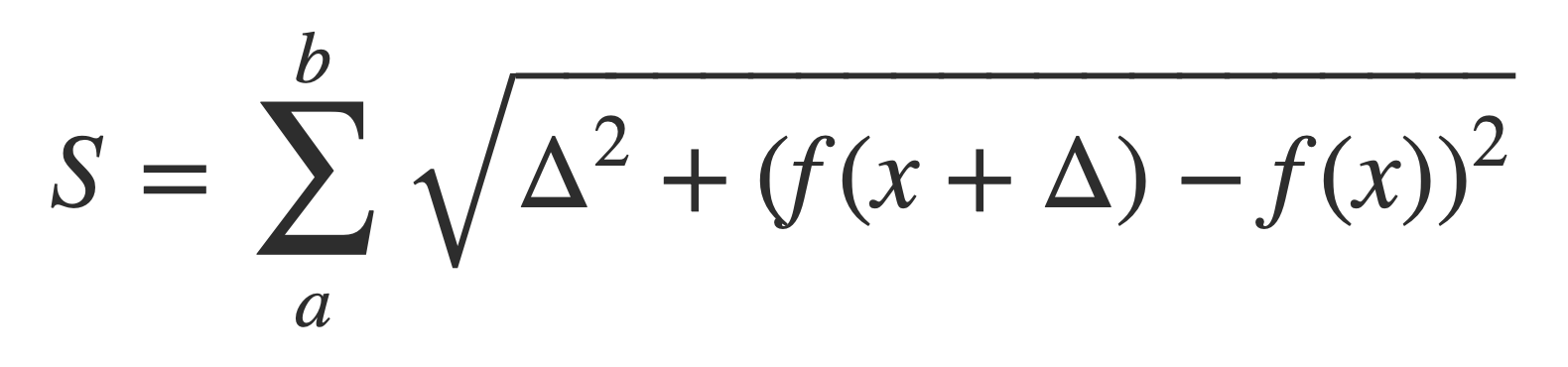
Factor out Δ2, then view this as a limit Δ -> 0:
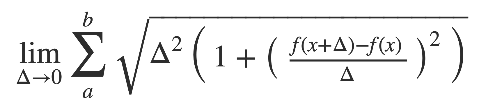
or
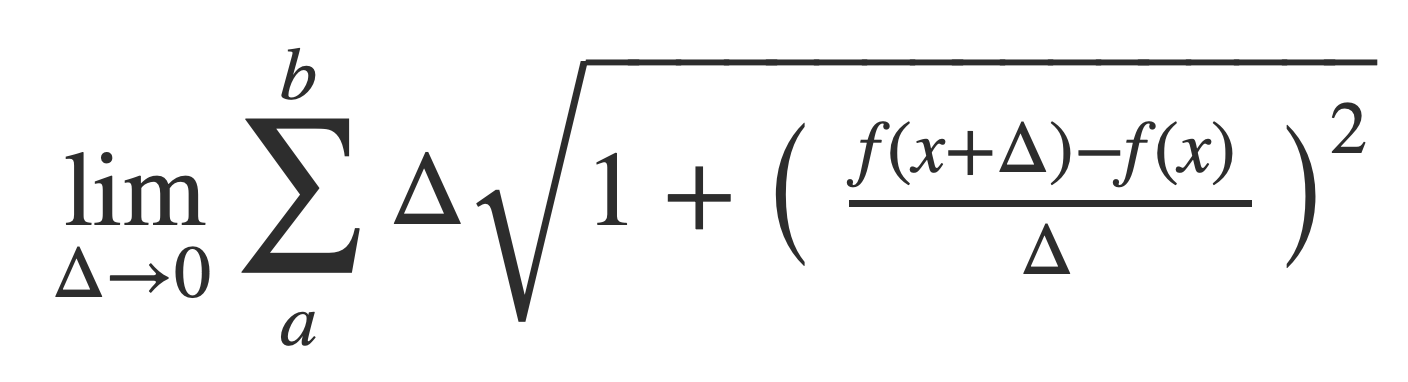
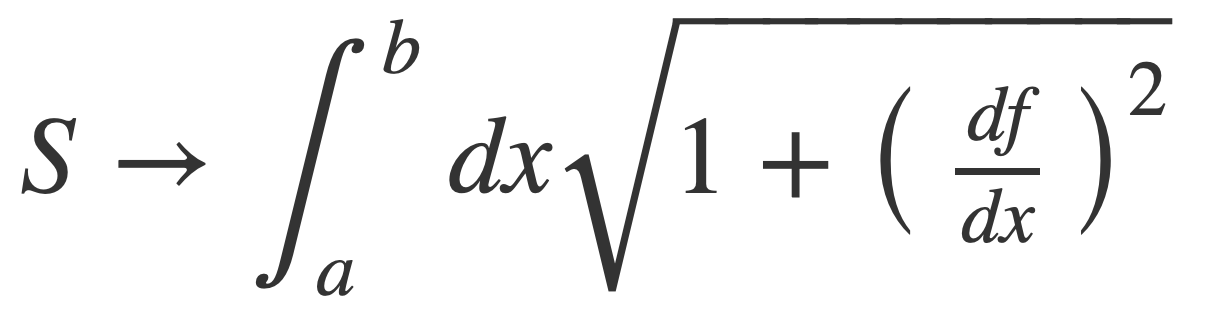
In the limit Δ -> 0 the sum becomes an integral and the ratio the derivative of the function f yielding a formula that defines the length of the path, or arc length:
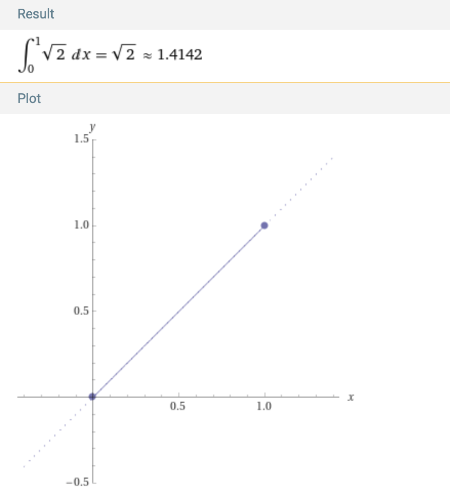
Example. The arc length of f(x) = x on [0,1] is the length of the diagonal of the unit square, or √2, using the Pythagorean theorem. Check this with the formula for arc length:
arclength x on 0,1
With the Pythagorean theorem and the definition of a circle as the set of points equidistant from a given point, the red semicircle path S of radius r = d/2 over the origin (0,0) is given by x2+y2 = r2:
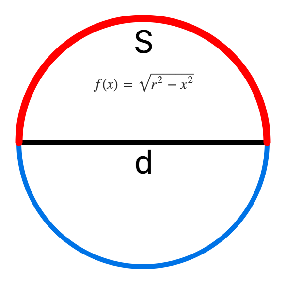
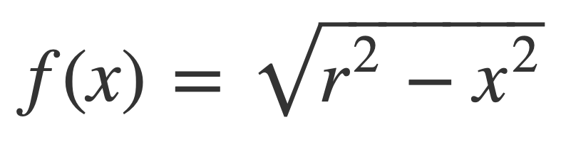
Solving for y provides the function f(x) for the path of the semicircle:
To find the arc length of S compute the derivative f’(x) = df/dx and square it:
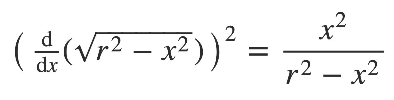
Substitute the derivative squared into the arc length formula:
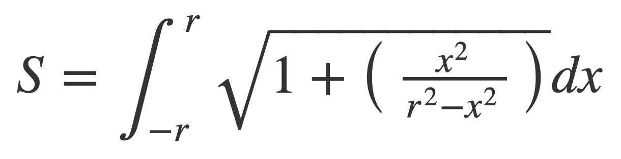
Using Change of Variables this expression for S can be written as the product of the radius r and an integral independent of r.
Change of Variables
The integral in the expression for S can be written as the product of the radius r and an integral independent of r with a substitution scale function g(x) = x r for x and application of the Change of Variables equation:
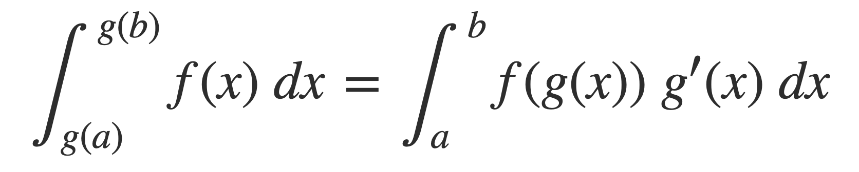
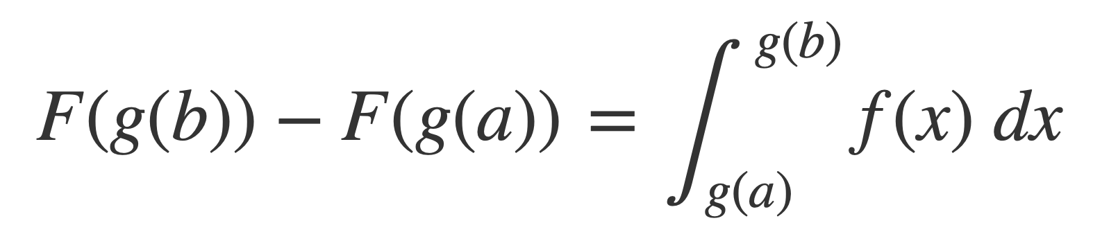
The Change of Variables equation is easy to check by applying the Fundamental Theorem of Calculus with the chain rule for the derivative for a composition of functions:
Let F be the antiderivative of f so that f = DF/dx.
Starting with the right hand side:
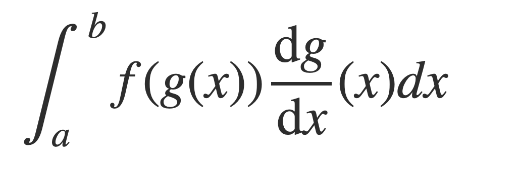
Substitute DF/dx for f, apply the chain rule for derivatives of composite functions, and then apply the Fundamental Theorem of Calculus:
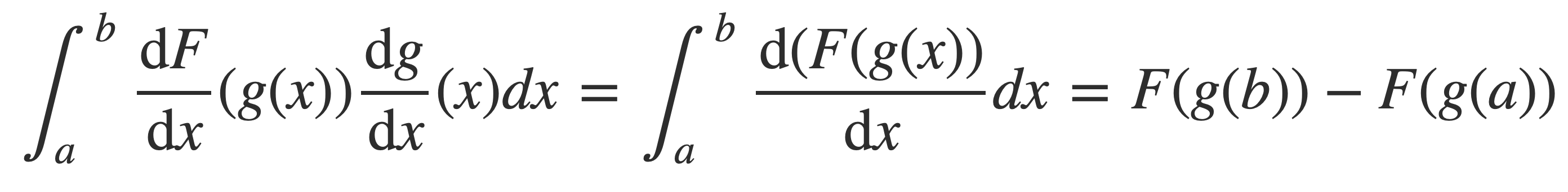
But again by the Fundamental Theorem of Calculus this is also the left hand side since f = DF/dx:
Apply Change of Variables to the formula for arc length by substituting g(x) = r x for x:
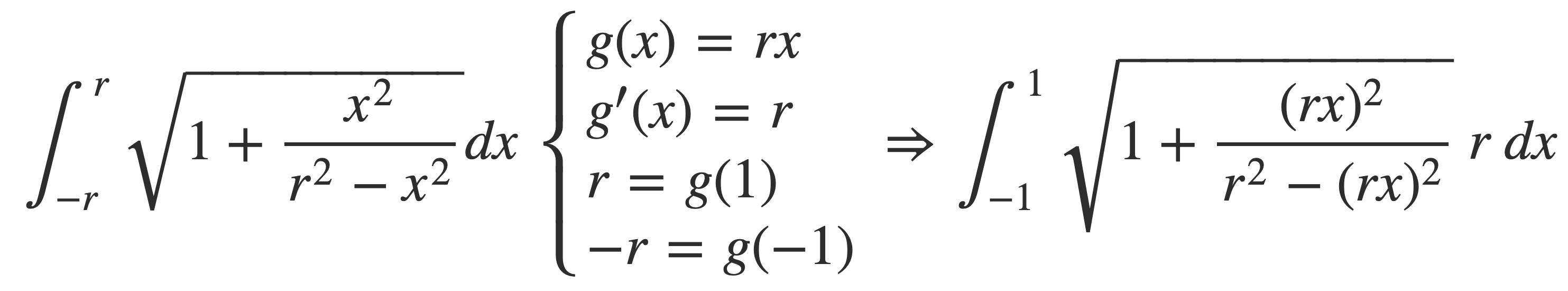
Move r outside the integral:
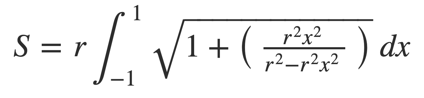
Simplify:
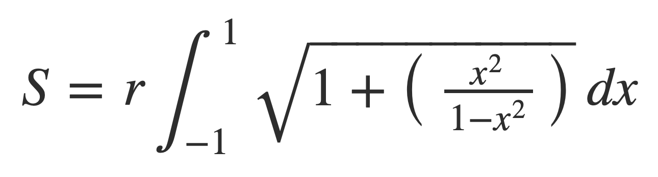
Simplify more:
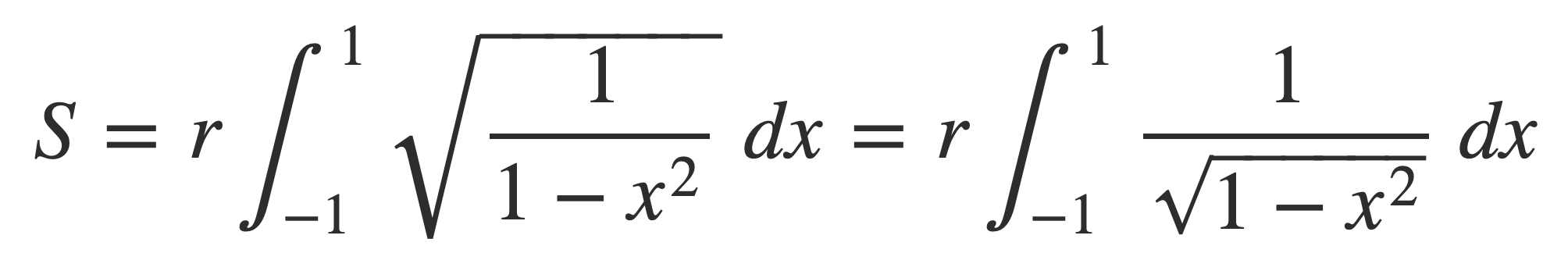
Now C/d is expressed by the following improper integral for circles of any radius r:
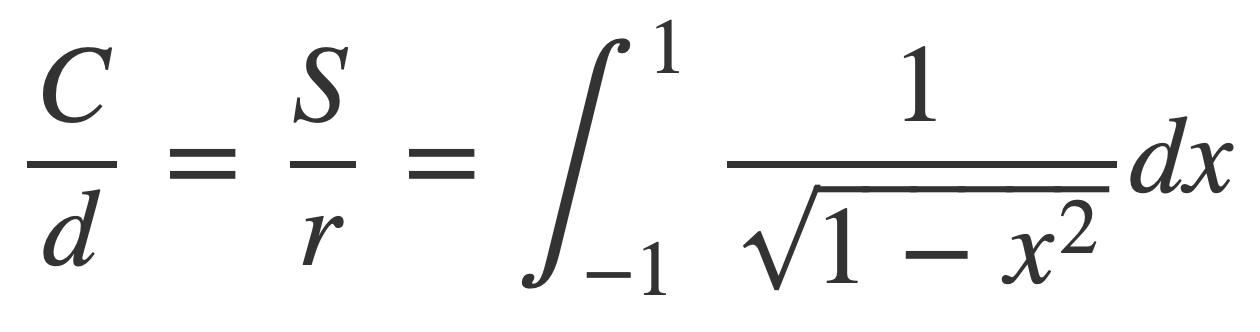
A plot of the integral:
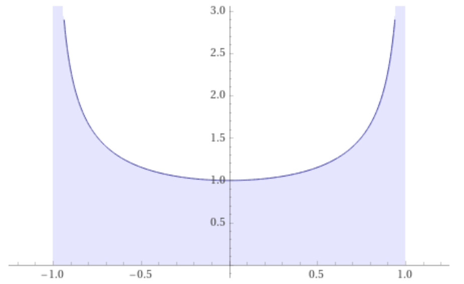
This is an improper integral because the integrand tends to ∞ at -1 and 1. Next it is shown that despite the singularities the value of the integral is finite, and its value C/d is the same for any circle.
Integral is Finite
The following integral, for π, is shown to be bounded.
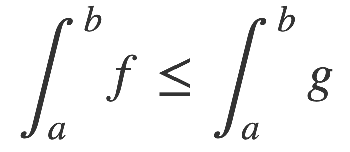
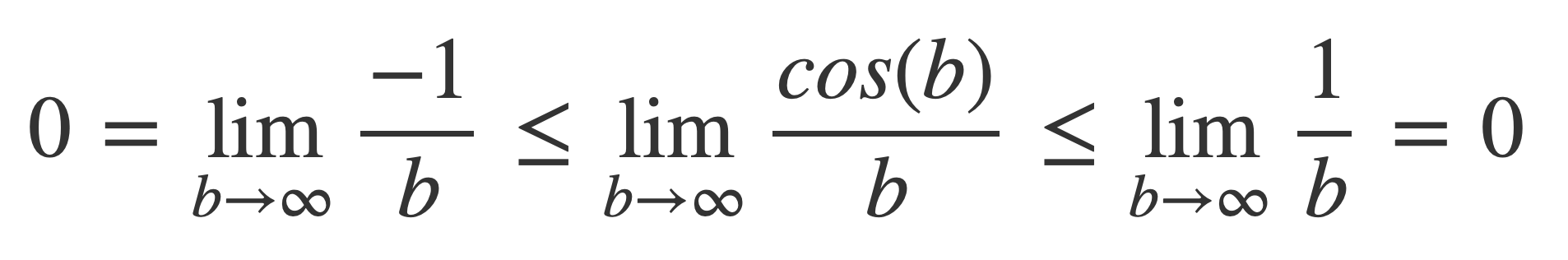
If for two integrable functions f,g it is true that f(x) ≤ g(x) for all x in the interval [a,b] then ∫ f-g = ∫ f - ∫ g ≤ 0, or:
Using the Fundamental Theorem of Calculus, and employing limits since the integrand is not differentiable at 0:
By symmetry and factoring:
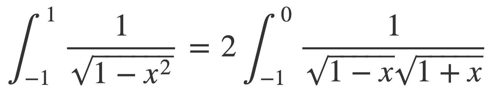
Since 1-x ≥ 1 on [-1,0]:
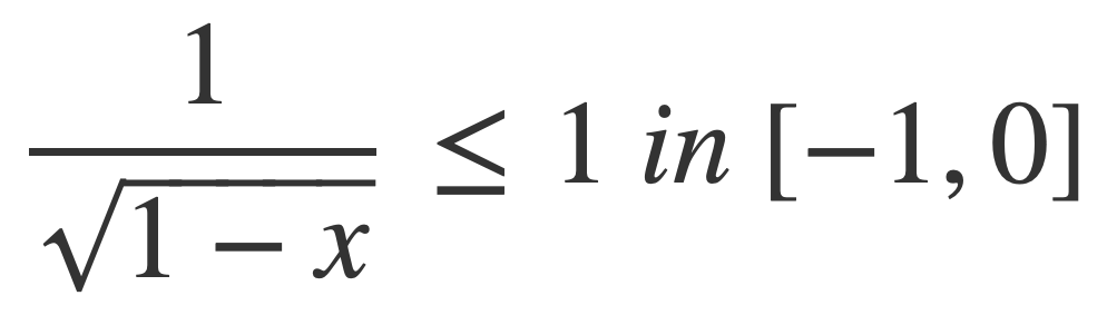
Using this inequality and that f ≤ g implies ∫ f ≤ ∫ g the integral can be bounded:
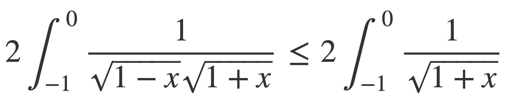
Now using the change of variables with g(x) = x-1, g’(x) = 1, g(0) = -1, g(1) = 0:
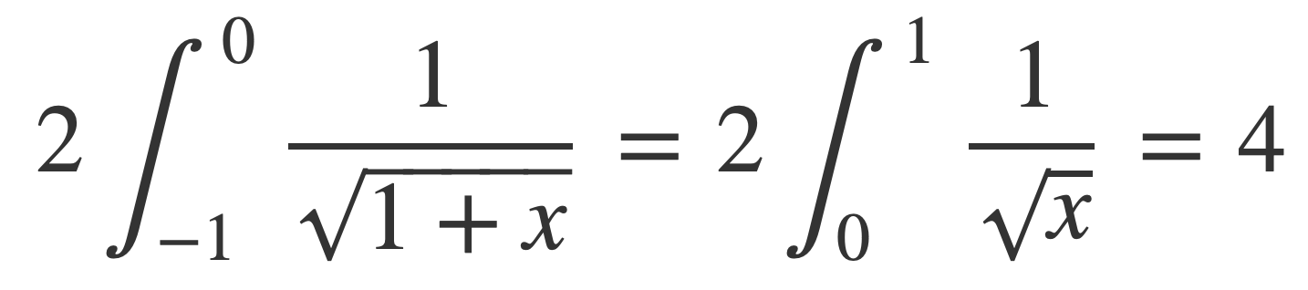
This means the integral for π exists and is bounded by 4:
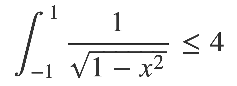
Therefore C/d is given by an integral whose value is independent of the radius, or the same for any circle.
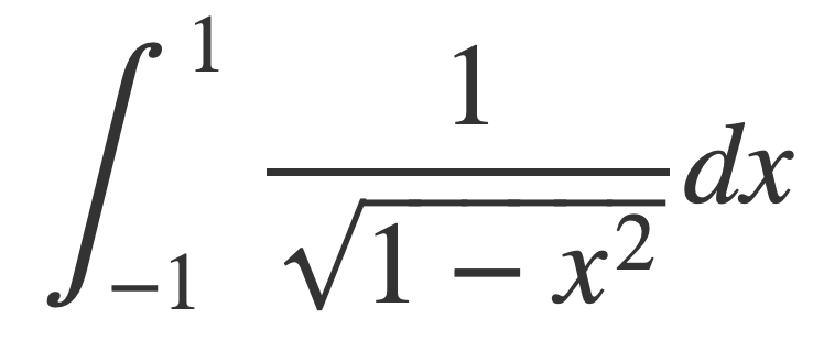
Compute π
As an aside, the value of the improper integral for C/d can be obtained by entering this expression:
Integrate[Divide[1,Sqrt[1-Power[x,2]]],{x,-1,1}]
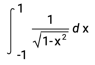
The integral evaluates to π:
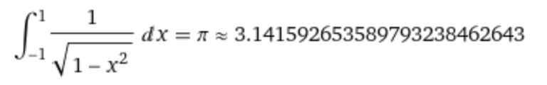
A plot of the integral:
Addendum About Sinc
Extrema of Sinc
A property of the sinc function is that the plot of sin(t)/t intersects the cosine function cos(t) at all of its extrema.
The extrema occur where the derivative is 0:
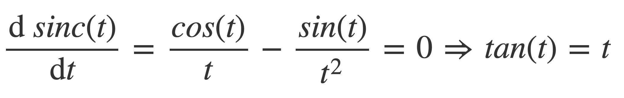
Solving for t yields tan(t) = sin(t)/cost(t) = t, or when sin(t)/t = cos(t)
Sinc is Integrable
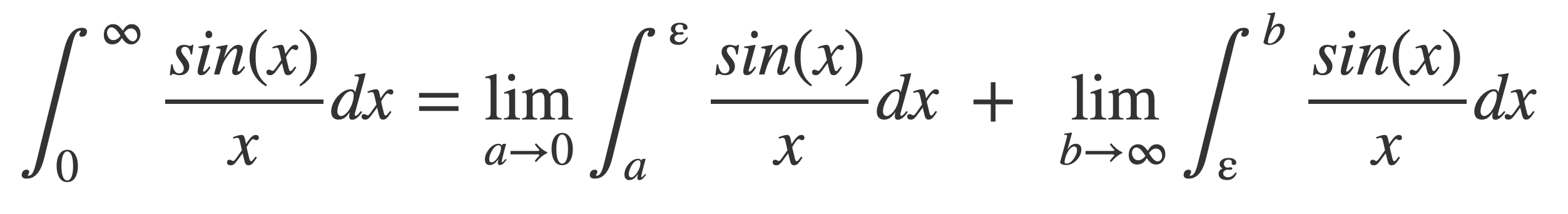
Because sinc is symmetric it only needs to be shown that the half integral on the right here, or Dirichlet integral, is integrable:
Partition the half integral on the right with some ε, 0 < ε < ∞, and then show each part is finite:
Apply the integration by parts formula
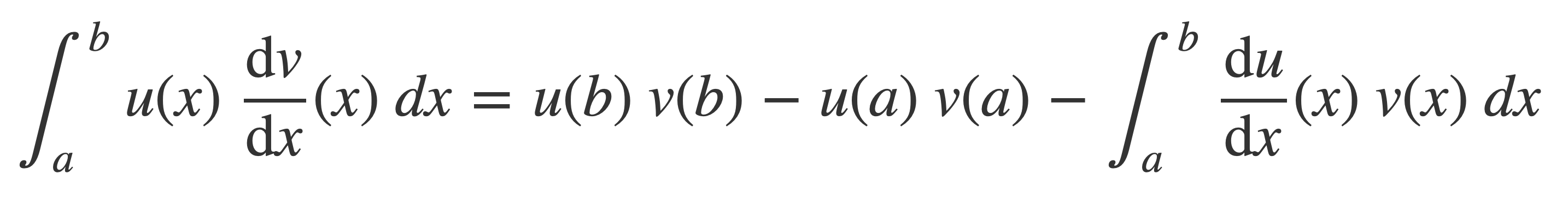
to obtain
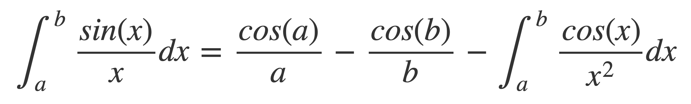
With this last expression, use the left hand side to investigate the limit a → 0+ and the right side for the limit b → ∞.
The left hand side integral is finite for non-zero b < ∞ as a → 0+, since by L’Hôpital’s Rule, for the integrand near 0:
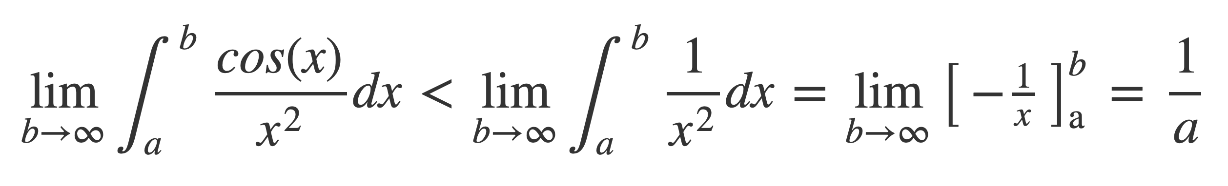
Now investigate the right side when 0 < a < ∞ as b → ∞.
This limit is 0:
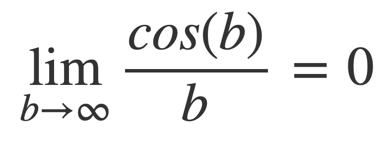
Since it is bounded on both sides by expressions that tend to 0 as b → ∞:
Also, the right hand side integral is finite because this integral is bounded:
Since both terms of the partitioned half integral were shown to be finite the sinc function is integrable.
Sinc is not Absolutely Integrable
For |sinc(x)|= |sin(x)/x|:
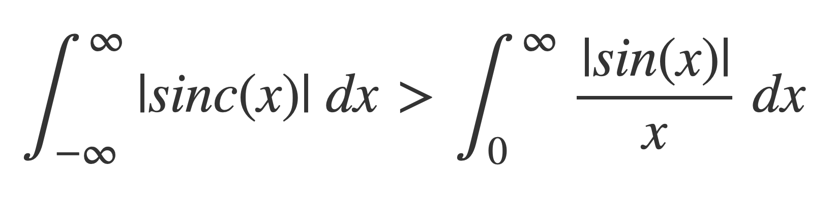
The integral on the right side can be shown to be infinite by writing it as an infinite sum of integrals over a partition of intervals [nπ, (n+1)π]:
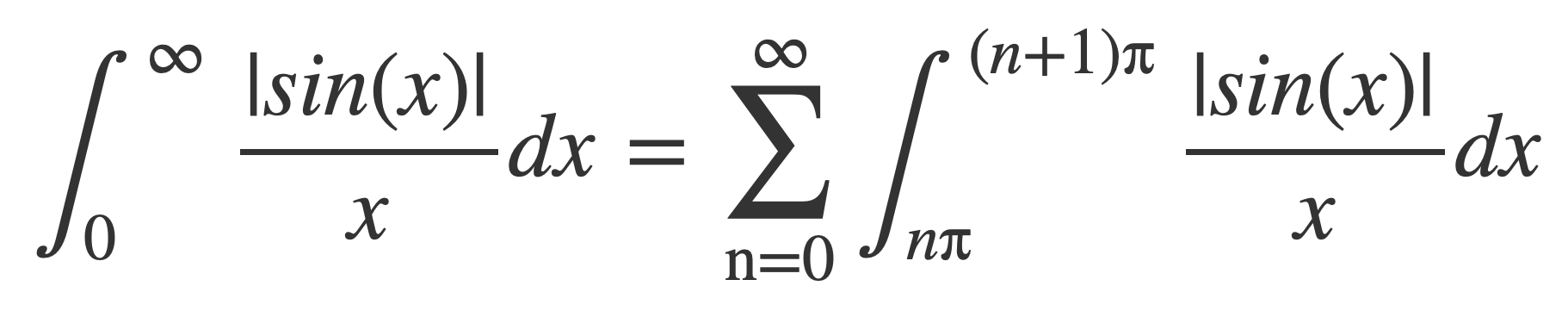
Because 1/x is decreasing on [nπ, (n+1)π] and therefore 1/x > 1/(n+1)π on [nπ, (n+1)π], each integral in the summation is bounded below, and so:
Replace each integral of |sin(x)| on the right by 2, since by periodicity they are all equal to the value of the following integral, which is 2:
The following integral on the left must be infinite because it is greater than the series on the right, and a harmonic series is divergent:
Fourier transform of Sinc
The following transform pairs are derived for the sinc function sinc and rectangle function rect:
![]()
and
![]()
The Fourier transform of the rectangle function rect(t) is computed first, and then the Fourier transform of sinc is computed using the duality and time scaling properties of the Fourier transform.
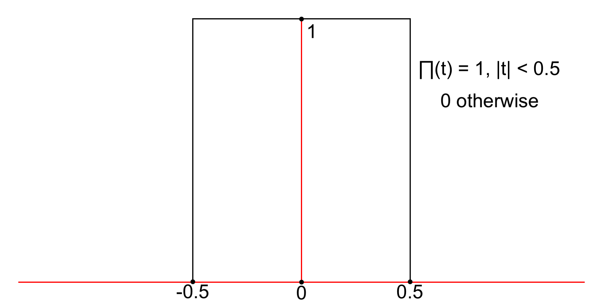
Compute the Fourier transform of the rectangle function rect(t) (also denoted by ∏):
![]()
Simplify using Euler’s Formula to convert to an expression with sinc:
![]()
The Fourier transform of the rect function is:
![]()
Check by entering this expression:
FourierTransform rect(t)
The result is, (∏(t) = rect(t)):
![]()
Plot of the Fourier transform of rect:
![]()
By duality, 𝓕[F(t)](ω) = f(-ω):
![]()
Pull out the factor √2√π:
![]()
Apply time scaling, with k = 2:
![]()
The Fourier transform of the sinc function is:
![]()
Check by entering this expression:
FourierTransform sinc(t)
The result is, (∏(t) = rect(t)):
![]()
Plot of the Fourier transform of sinc:
![]()
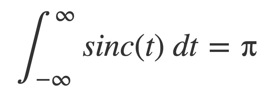
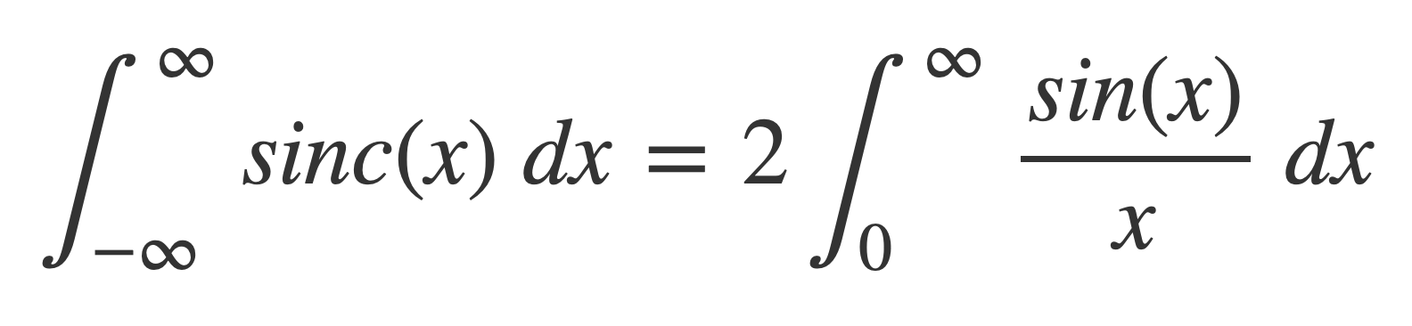
Integration of Sinc
The value of the improper integral of the sinc function is twice the value of the Dirichlet integral:
In Dirichlet integral it is noted that it can be computed in numerous ways, but the Fourier transform of sinc provides the answer too.
The value of the integral of the sinc function, shown to exist in Sinc is Integrable, is obtained using the value of its Fourier transform at ω = 0:
![]()
The value is π: